ridge = {

  // Set up SVG dimensions
  const svgWidth = 490;
  const svgHeight = 400;
  const margin = { top: 10, right: 10, bottom: 10, left: 10 };
  const width = svgWidth - margin.left - margin.right;
  const height = svgHeight - margin.top - margin.bottom;

  // Create an SVG container
  const svg = d3.create("svg")
    .attr("width", svgWidth)
    .attr("height", svgHeight);
  var e = s/2;
  var ellipsesData = [
      { cx: 250, cy: 190, rx: 199, ry: 68, angle: 40 },
      { cx: 250, cy: 190, rx: 32, ry: 20, angle: 40 },
      { cx: 250, cy: 190, rx: 200 - 1.68*s, ry: 68- 0.48*s, angle:  40  , style: "black" }
  ];

  // Define circle data
  const circleData = [
  { cx:150, cy: 260, r: 50 + e, color: "black" }
  ];

  // Create circles
  svg.selectAll("circle")
    .data(circleData)
    .enter()
    .append("circle")
    .attr("cx", d => d.cx)   // x-coordinate of the center
    .attr("cy", d => d.cy)   // y-coordinate of the center
    .attr("r", d => d.r)     // radius
    .attr("stroke", d => d.color)
    .style("fill", "lightgrey");// fill color


// Function to create arrowheads
  function createArrowhead(id, orientation) {
    svg.append("defs").append("marker")
    .attr("id", id)
    .attr("refX", 6)
    .attr("refY", 6)
    .attr("markerWidth", 10)
    .attr("markerHeight", 10)
    .attr("orient", orientation)
    .append("path")
    .attr("d", "M2,2 L6,6 L2,10 L10,6 L2,2")
    .style("fill", "grey");
  }

  // Create arrowheads for different directions
  createArrowhead("arrowhead-left", 180);
  createArrowhead("arrowhead-right", 0);
  createArrowhead("arrowhead-up", 270);
  createArrowhead("arrowhead-down", 90);

  // Render X and Y axes
  svg.append("line")
      .attr("x1", 20)
      .attr("y1", 260)
      .attr("x2", 480)
      .attr("y2", 260)
      .style("stroke", "grey")
      .attr("marker-start", "url(#arrowhead-left)")
      .attr("marker-end", "url(#arrowhead-right)");

  svg.append("line")
      .attr("x1", 150)
      .attr("y1", 50)
      .attr("x2", 150)
      .attr("y2", 380)
      .style("stroke", "grey")
      .attr("marker-start", "url(#arrowhead-up)")
      .attr("marker-end", "url(#arrowhead-down)")

  // Add "beta2" beside the Y-axis
  svg.append("text")
    .attr("x", 130) // Adjust the x-coordinate for positioning
    .attr("y", 50) // Adjust the y-coordinate for positioning
    .style("fill", "black")
    .style("font-size", "14px")
    .text("β")
    .append("tspan")
    .attr("dy", "0.5em")
    .attr("font-size", "0.8em")
    .text("2");

  // Add "beta1" beside the X-axis
    svg.append("text")
      .attr("x", 480) // Adjust the x-coordinate for positioning
      .attr("y", 275) // Adjust the y-coordinate for positioning
      .style("fill", "black")
      .style("font-size", "14px")
      .text("β")
      .append("tspan")
      .attr("dy", "0.5em")
      .attr("font-size", "0.8em")
      .text("1");
    // Add "beta1" beside the X-axis
    svg.append("text")
      .attr("x", 540) // Adjust the x-coordinate for positioning
      .attr("y", 275) // Adjust the y-coordinate for positioning
      .style("fill", "black")
      .style("font-size", "14px")
      .text("β")
      .append("tspan")
      .attr("dy", "0.5em")
      .attr("font-size", "0.8em")
      .text("1");

  svg.selectAll("ellipse")
    .data(ellipsesData)
    .enter()
    .append("ellipse")
    .attr("cx", function (d) { return d.cx; })
    .attr("cy", function (d) { return d.cy; })
    .attr("rx", function (d) { return d.rx; })
    .attr("ry", function (d) { return d.ry; })
    .attr("transform", function (d) {
        return "rotate(" + d.angle + " " + d.cx + " " + d.cy + ")";
    })
    .style("fill", "none")
    .style("stroke", function (d) { return d.style || "#336699"; }); // Use "black" if style is defined, otherwise use "#336699"

  // Make the #e52320 dotted line
  svg.append("line")
    .attr("x1", 187)
    .attr("y1", 223)
    .attr("x2", 248)
    .attr("y2", 188)
    .style("stroke", "#e52320")
    .style("stroke-width", 3)
    .style("stroke-dasharray", "3,3");

  // Make dot at the center
  svg.selectAll("dot")
    .data(ellipsesData)
    .enter()
    .append("circle")
    .attr("cx", function (d) { return d.cx -2; })
    .attr("cy", function (d) { return d.cy - 2; })
    .attr("r", 3) // Radius of the dot
    .style("fill", "black");

  // Add "OLS" label beside the dots
  svg.selectAll("label")
    .data(ellipsesData)
    .enter()
    .append("text")
    .attr("x", function (d) { return d.cx + 5; }) // Adjust the x-coordinate for positioning
    .attr("y", function (d) { return d.cy; })
    .text("OLS")
    .style("fill", "black")
    .style("font-size", "10px");

  // Make dot for the smallest ellipse
  svg.selectAll("dot")
    .data(ellipsesData)
    .enter()
    .append("circle")
    .attr("cx", 187 + 0.43*s)
    .attr("cy", 223 - 0.26*s )
    .attr("r", 3) // Radius of the dot
    .style("fill", "#336699");

  return svg;
}

lasso = {

  const svgWidth = 490;
  const svgHeight = 400;
  const margin = { top: 10, right: 10, bottom: 10, left: 10 };
  const width = svgWidth - margin.left - margin.right;
  const height = svgHeight - margin.top - margin.bottom;

  const svg = d3.create("svg")
    .attr("width", svgWidth)
    .attr("height", svgHeight);

  var a =0;
  var b =0;
  var c =1;
  var d =1;;

  if(s <= 50){
    a = s;
    b = 0;
    c = 1;
    d = 0;
  } else {
    a = 0;
    b = s - 50;
    c = 0;
    d = 1;
  }

  var ellipsesData = [
    { cx: 300, cy: 200, rx: c*180 - 0.22*2*a, ry: c*51- 0.28*2*a, angle: 16 + 0.03*2*a },
    { cx: 300, cy: 200, rx: d*158 - 0.5*2*b, ry: d*23- 0.14*2*b, angle: 19 },
  ];

  // svg.append("text")
  //   .attr("x", 350)
  //   .attr("y", 70)
  //   .style("fill", "black")
  //   .style("font-size", "14px")
  //   .text(`RSS = ${2600 - s*s/4}`);


  // Dimensions of the square
  const squareSize = 100 + s;

  // center of the square
  const centerX = 150;
  const centerY = 260;

  const squareGroup = svg.append("g")
    .attr("transform", `translate(${centerX}, ${centerY})`);

  squareGroup.append("rect")
    .attr("x", -squareSize / 2)
    .attr("y", -squareSize / 2)
    .attr("width", squareSize)
    .attr("height", squareSize)
    .attr("transform", "rotate(45)")
    .style("stroke", "black")
    .style("fill", "lightgrey");

// Function to create arrowheads
  function createArrowhead(id, orientation) {
    svg.append("defs").append("marker")
      .attr("id", id)
      .attr("refX", 6)
      .attr("refY", 6)
      .attr("markerWidth", 10)
      .attr("markerHeight", 10)
      .attr("orient", orientation)
      .append("path")
      .attr("d", "M2,2 L6,6 L2,10 L10,6 L2,2")
      .style("fill", "grey");
  }

  // arrowheads for different directions
  createArrowhead("arrowhead-left", 180);
  createArrowhead("arrowhead-right", 0);
  createArrowhead("arrowhead-up", 270);
  createArrowhead("arrowhead-down", 90);

  // Render X and Y axes
  svg.append("line")
    .attr("x1", 5)
    .attr("y1", 260)
    .attr("x2", 480)
    .attr("y2", 260)
    .style("stroke", "grey")
    .attr("marker-start", "url(#arrowhead-left)")
    .attr("marker-end", "url(#arrowhead-right)");

  svg.append("line")
    .attr("x1", 150)
    .attr("y1", 50)
    .attr("x2", 150)
    .attr("y2", 410)
    .style("stroke", "grey")
    .attr("marker-start", "url(#arrowhead-up)")
    .attr("marker-end", "url(#arrowhead-down)")

  svg.append("text")
    .attr("x", 130)
    .attr("y", 50)
    .style("fill", "black")
    .style("font-size", "14px")
    .text("β")
    .append("tspan")
    .attr("dy", "0.5em")
    .attr("font-size", "0.8em")
    .text("2");

  svg.append("text")
    .attr("x", 480)
    .attr("y", 275)
    .style("fill", "black")
    .style("font-size", "14px")
    .text("β")
    .append("tspan")
    .attr("dy", "0.5em")
    .attr("font-size", "0.8em")
    .text("1");

  svg.append("text")
    .attr("x", 540)
    .attr("y", 275)
    .style("fill", "black")
    .style("font-size", "14px")
    .text("β")
    .append("tspan")
    .attr("dy", "0.5em")
    .attr("font-size", "0.8em")
    .text("1");

  svg.selectAll("ellipse")
    .data(ellipsesData)
    .enter()
    .append("ellipse")
    .attr("cx", function (d) { return d.cx; })
    .attr("cy", function (d) { return d.cy; })
    .attr("rx", function (d) { return d.rx; })
    .attr("ry", function (d) { return d.ry; })
    .attr("transform", function (d) {
        return "rotate(" + d.angle + " " + d.cx + " " + d.cy + ")";
    })
    .style("fill", "none")
    .style("stroke", function (d) { return d.style || "#336699"; });

  // Make dot at the center
  svg.selectAll("dot")
    .data(ellipsesData)
    .enter()
    .append("circle")
    .attr("cx", function (d) { return d.cx; })
    .attr("cy", function (d) { return d.cy; })
    .attr("r", 3) // Radius of the dot
    .style("fill", "black");

  // Add "OLS" label beside the dots
  svg.selectAll("label")
    .data(ellipsesData)
    .enter()
    .append("text")
    .attr("x", function (d) { return d.cx + 5; })
    .attr("y", function (d) { return d.cy; })
    .text("OLS")
    .style("fill", "black")
    .style("font-size", "10px");

  svg.append("line")
    .attr("x1", 150)
    .attr("y1", 153)
    .attr("x2", 150)
    .attr("y2", 260)
    .style("stroke", "#e52320")
    .style("stroke-width", 3)
    .style("stroke-dasharray", "3,3");

  svg.append("line")
    .attr("x1", 150)
    .attr("y1", 153)
    .attr("x2", 300)
    .attr("y2", 200)
    .style("stroke", "#e52320")
    .style("stroke-width", 3)
    .style("stroke-dasharray", "3,3");

  svg.selectAll("dot")
    .data(ellipsesData)
    .enter()
    .append("circle")
    .attr("cx", 150)
    .attr("cy", 188 - 0.35*2*a )
    .attr("r", 3*c)
    .style("fill", "#336699");

  svg.selectAll("dot")
    .data(ellipsesData)
    .enter()
    .append("circle")
    .attr("cx", 150 + 0.47*2*b)
    .attr("cy", 153 + 0.14*2*b )
    .attr("r", 3*d)
    .style("fill", "#336699");

  return svg;
}Supervised Machine Learning
An Introduction using Decision Tree Learning
Introduction
What the fuzz is about
What is Machine Learning?
- Pattern recognition: abstraction of patterns and regularities from data
- Predictive modelling: optimized prediction of outcome given a set of inputs
- Broad range of methods and models
- Methods are often a “black box” compared to estimating causal effects
- Often used synonymously with artificial intelligence (AI)
Branches of Machine Learning
- Supervised learning:
- Data set already contains values for outcomes
- Parameters are optimized in a training data set in such a way that the predictions are as “accurate” as possible in a test data set
- e.g., decision trees, linear models with regularization term, neural networks, etc.
- Unsupervised learning:
- There is no predetermined classification or measure of some outcome variable
- Rather the algorithm comes up with a systematization of the input data (“speaks to us”)
- e.g., principal component analysis, clustering algorithms, etc.
- Reinforcement learning:
- The algorithm is rewarded by ending up in a “good spot” and subsequently chooses the best path through the game
- e.g., robotic movement, gaming, etc.
Supervised Learning in a Nutshell
- An outcome is to be predicted
- Continuous outcome → regression problem
- Discrete outcome → classification problem
- Outcome for a set of input variables (features) is known (labelled/annotated)
- Is split into training and test data
- Model is fit into training data
- Performance is evaluated in test data
- Parameters are chosen to optimize performance
- Model can be used to predict in new data
Uses of Machine Learning
- Spam filter
- Recommender systems
- Optical character recognition
- Natural language processing
- Data imputation
- Prediction models in science
- Statistical profiling
Classification and Regression Trees
A simple and powerful algorithm to understand
CART
- CART (Classification and Regression Trees) methodology by Leo Breiman (1984)
- Algorithmically: Use of binary decision rules for dealing with classification and regression problems
- Geometrically: Partitioning of the support space spanned by a set of predictors
- Statistically: Assigning an outcome by fitting a very simple function (a piecewise constant) over partitions
Tree Graph and Partitioning of the Support Space


Tree Graph and Regression Line


Classification Problem
- For a discrete response, the underlying minimization problem can be written as:
\[ \min_{R_t} \left\{ \sum_{t=1}^{T} w_t \cdot G_{R_t} + C(\lambda, T) \right\} \]
-
- \(R_t\) is the partition on the support corresponding to the \(t\)-th terminal node
- \(T\) is the number of terminal nodes of the tree
- \(w_t\) is the fraction of observations in the \(t\)-th terminal node
- \(G_{R_t}\) is the Gini impurity for partition \(R_t\) / the \(t\)-th terminal node
- \(C(\lambda, T)\) is some cost function, sometimes called a regularization term
- (\(\lambda\) is the tuning parameter that decides the complexity of the model by adding cost)
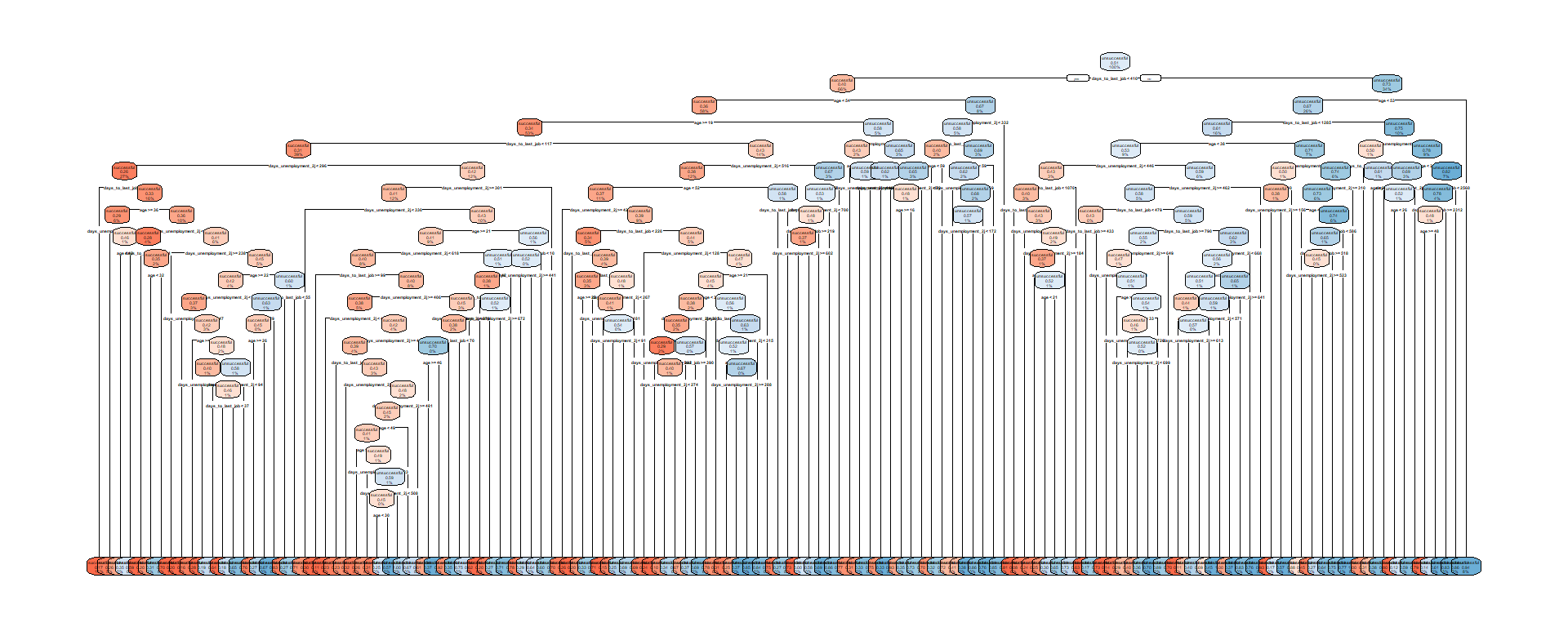
Example of Gini Impurity
- The Gini impurity is a measure of information given by \[ G = 1 - \sum_{j=1}^{J} p_j^2 \]
- Where \(p_j\) is the fraction of class \(j\)
- Looking at the first node from the classification tree from before, we obtain \[ G = 1 - 0.49^2 - 0.51^2 = 0.4998 \]
- By splitting at the first node we get a weighted impurity of \[ G = 0.56*(1 - 0.37^2 - 0.63^2) + 0.44*(1 - 0.66^2 - 0.34^2) = 0.4585 \]
- In the terminal nodes we end up with a weighted Gini impurity of: \[ G = 0.47*(1 - 0.32^2 - 0.68^2) + 0.06*(1 - 0.58^2 - 0.42^2) + ... = 0.4484 \]
Regression Problem
For a continuous response, the underlying minimization problem can be written as
\[ \min_{R_t} \left\{ \; \sum_{t=1}^{T} \sum_{x_i \in R_t} (y_i - \overline{y}_{R_t})^2 \; + \; {C}(\lambda,T) \right\} \]
where \(\overline{y}_{R_t}\) is the mean of the variables in partition \(R_t\)
Algorithm I
- How are the partitions \(R_t\) determined?
- Beginning from the first node, each split is determined by the variable and value which minimizes the RSS (regression problem) or impurity (classification problem)
- End up with the most complex tree explaining every data point
- Pruning the tree
- Pre-pruning: additional splits are created until cost of depth is too high
- Post-pruning: complex tree is created and cut down to a size where cost is met
- Post-pruning is preferred because stopping too early bears the danger of missing some split down the line
Algorithm II
- How is the tuning parameter \(\lambda\) determined?
- Employing cross-validation, we choose the parameter value which minimizes some prediction error in the test/validation data (more on that later)
- Exact implementation of the algorithm differs
- Different packages may use different impurity/information measures (e.g., entropy) and different cost functions/tuning parameters
- e.g.,
rpartuses post-pruning where the complexity parametercpregulates the minimum gain in \(R^2\) or minimum decrease of Gini impurity to create another node
Growing the Tree


Advantages and Drawbacks
- Trees have many advantages
- Easy to understand and very flexible
- No theoretical assumptions needed
- Computationally cheap
- Automatic feature selection
- No limitation in number of features
- Do not necessarily discard observations
- Drawbacks include
- No immediate (causal) interpretation of decision
- Algorithm is “greedy”
- The curse of dimensionality
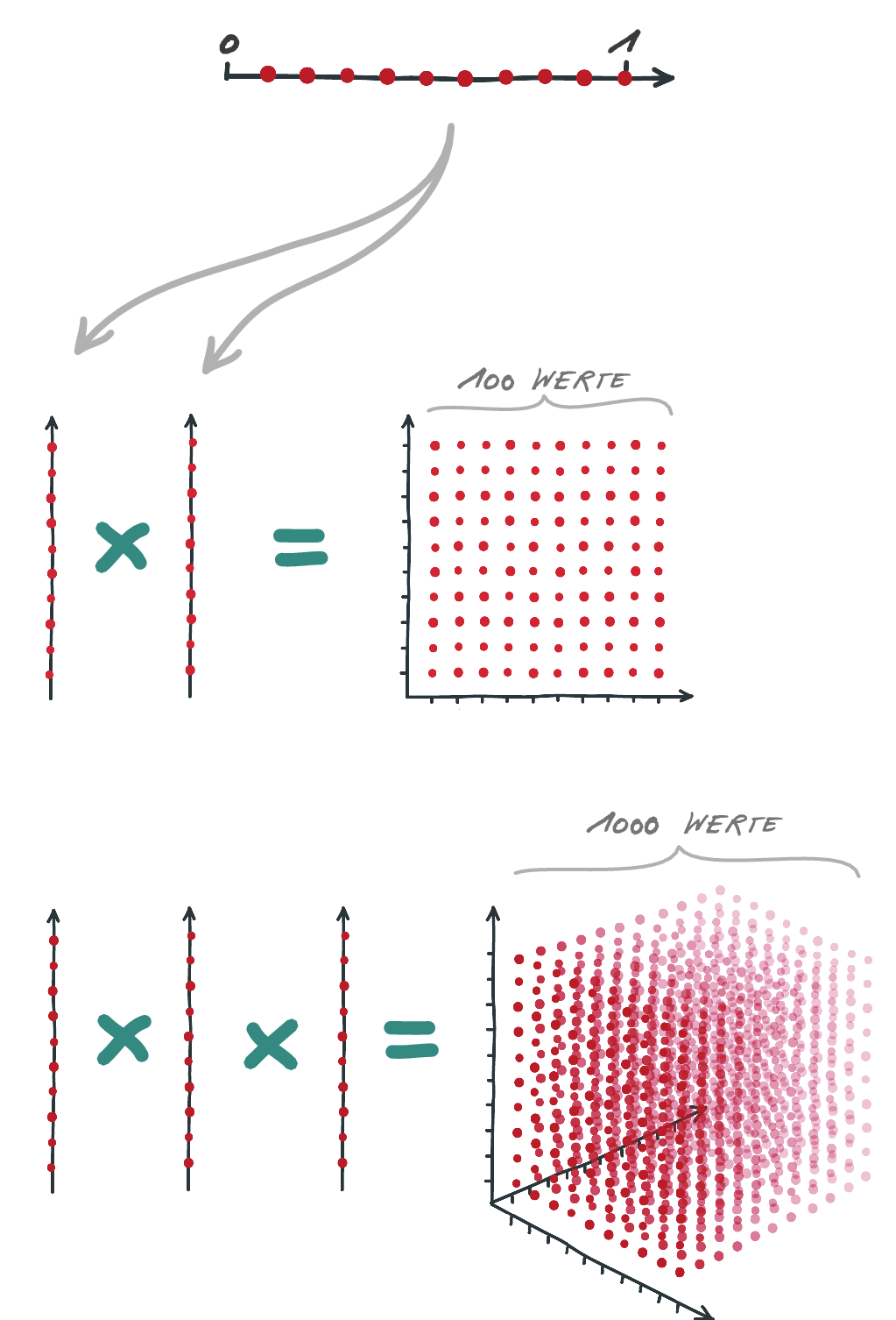
The Curse of Dimensionality
- Volume of the support space increases exponentially with dimensions
- Data points become dispersed in a high-dimensional space
- Splits become very volatile
- To mitigate the problem, random forest is used in practice
A Perfect Summary I

Performance Measurement
Connecting to statistical theory
Root Mean Squared Error
- For a regression problem, RMSE is typically used: \[ RMSE = \sqrt{\frac{1}{n}\sum_{i=1}^{n}(y_{i} - \hat{y}_{i})^{2}} \]
- Or alternatively the (adjusted) \(R^2\): \[ R^2 = 1 - \frac{\sum_{i=1}^{n}({y_i}-\hat{y_i})^2}{\sum_{i=1}^{n}(y_i-\bar{y})^2} \]
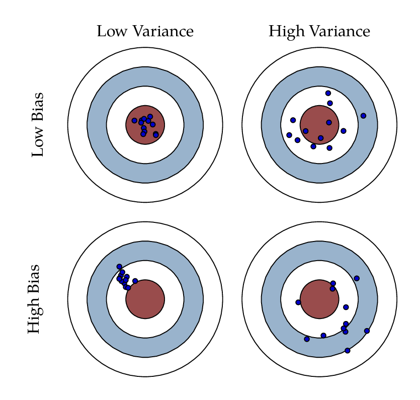
Bias–Variance Trade-Off
- The mean squared error \(MSE\) of a prediction can be written as:
\[ MSE(y, \hat{f}(x)) = \mathbb{E}\left[(y - \hat{f}(x))^2\right] \]
- Where \(y = f(x) + \epsilon\) is the true data generating process and \(\mathbb{V}[\epsilon] = \sigma^2\) and \(\mathbb{E}[\epsilon] = 0\)
- And \(\hat{f}(x)\) is the function predicting \(y\) given predictors \(x\)
\[ MSE(y, \hat{f}(x)) = \underbrace{(\mathbb{E}[f(x) - \hat{f}(x)])^2}_{\text{bias}} + \underbrace{\mathbb{E}[\hat{f}(x) - \mathbb{E}(\hat{f}(x))]^2}_{\text{variance}} + \underbrace{\mathbb{E}[(y - f(x))^2]}_{\text{irreducible error}} = \]
\[ = \underbrace{\mathrm{bias}^2 + \mathrm{variance}}_{\text{reducible error}} + \sigma^2 \]
Trade-Off
- It is possible to specify \(\hat{{f}}(x)\) in such a way that introduces a bias but reduces the variance, so that the \(MSE\) reduces
- Notice that this is well in line with what we know from the theory of the linear model
- To exploit this trade-off in a linear model we can add a regularization term
Ridge Regression and LASSO
If we introduce the term \(\lambda \cdot || \beta ||_2\) into the well-known minimization task of a linear model, this is called ridge regression
\[\widehat{\beta}_{RIDGE} = \min_\beta \left\{ || y - X\beta ||_2 + \lambda \cdot || \beta ||_2 \right\}\]
- If we use the penalty \(\lambda \cdot || \beta ||_1\), we get the LASSO estimator
- As a result, the coefficients of our parameters (and in many cases the \(MSE\)) shrink towards zero
Properties of Shrinkage Estimators
- This can also be used as a method for variable selection
- Coefficients of variables with low predictive power shrink close to zero (\(\widehat{\beta}_{RIDGE}\)) or to zero (\(\widehat{\beta}_{LASSO}\))
- Introducing downward bias into coefficients \(\mathbb{E}\left[\widehat{\beta}_{RIDGE}\right] < \beta\)
- For large \(k\) and fixed \(n\) we often times observe \(MSE(y, \hat{f}_{RIDGE}(x)) < MSE(y, \hat{f}_{OLS}(x))\)
- For sample size \(n \to \infty\) and fixed number of coefficients \(k\) it holds that \(\widehat{\beta}_{RIDGE} = \widehat{\beta}_{OLS}\)
Coefficient Shrinkage
regularization term \(\lambda\) =
Confusion Matrix
- for a classification problem we can look at a confusion matrix
htl.html`
<div class="frame">
  <div class="table">
    <table width="1000px">
      <tr>
        <th></th>
        <th></th>
        <th colspan="2">Actual</th>
      </tr>
      <tr>
        <th></th>
        <th></th>
        <th>positive</th>
        <th>negative</th>
      </tr>
      <tr>
        <td rowspan="2" style="transform: rotate(-0deg);"><b>Predicted </b></td>
        <td><b>positive</b></td>
        <td style="background-color: rgba(0, 128, 0, 0.55);"># true positive (TP)</td>
        <td style="background-color: rgba(255, 0, 0, 0.55);"># false positive (FP)</td>
        <td><span class="formula">Precision = ${tex`\frac{TP}{TP+FP}`}</span></td>
      </tr>
      <tr>
        <td><b>negative</b></td>
        <td style="background-color: rgba(255, 0, 0, 0.55);"># false negative (FN)</td>
        <td style="background-color: rgba(0, 128, 0, 0.55);"># true negative (TN)</td>
        <td><span class="formula"> NPV = ${tex`\frac{TN}{TN+FN}`}</span></td>
      </tr>
      <tr>
        <td></td>
        <td></td>
        <td><span class="formula">Sensitivity = ${tex`\frac{TP}{TP+FN}`}</span></td>
        <td><span class="formula">Specificity = ${tex`\frac{TN}{TN+FP}`}</span></td>
        <td><span class="formula">Accuracy = ${tex`\frac{TP+TN}{n}`}</span></td>
      </tr>
    </table>
  </div>
</div>
`
Base-Rate Fallacy
- Beware of the base rate fallacy:
- Let’s assume the Austrian population is getting tested for the Coronavirus
- 1% of the population is indeed infected, meaning \(P(C) = 0.01\)
- A test is 98% accurate, in the sense that \(P(\text{Test}_C \mid C) = P(\text{Test}_{\neg C} \mid \neg C) = 0.98\)
- What is the probability that I have the Coronavirus given that I tested positive? \(P(C \mid \text{Test}_C)\)?
- Which value from the confusion matrix did we calculate here (and which ones were given)?
Judging Performance in Classification Problems
- All the indicators in the confusion matrix can be relevant
- Accuracy depends on base rate
- accuracy of 96% in sample with 95% positives → poor performance
- accuracy of 80% in sample with 50% positives → good performance
- Need for adjustment of values relative to a “naive prediction”
- Concepts can be generalized to classification problems with more than two categories
Adjusted Performance Measures
- Cohen’s kappa: \[ \kappa = \frac{Acc_{mod} - Acc_{0}}{1 - Acc_{0}} \] where \(Acc_{mod}\) is the accuracy of our model and \(Acc_{0}\) is the expected random accuracy
For any sensible model, it holds that \(0 < \kappa < 1\)
If \(\kappa < 0\), our model would be worse than guessing at random
\(\kappa\) tells you “how far you are away from predicting perfectly compared to a naive prediction”
ROC- and PR-Curve
- Trade-off between the measures, which we can exploit by setting the cut-off point for predicted scores
- Receiver Operating Characteristic (ROC) curve
- Plot of sensitivity against 1-specificity
- Helps identify which cut-off point to choose
- Precision-Recall (PR) curve
- Plot of precision against sensitivity (recall)
- Might be preferred over ROC when categories are very imbalanced
Receiver Operating Characteristic
- The trade-off through the setting of the cut-off point can be visualized in a ROC curve

Receiver Operating Characteristic
- ROC criterion
- There is a point on the curve where the loss of sensitivity and specificity are equal
- This value can be used to determine an “optimal” cut-off point
- Sometimes high sensitivity is preferred over specificity (e.g., medical tests), or vice versa
- Area Under the Curve (AUC)
- The area underneath the ROC curve can be used as another performance measure
- Different models achieve different sensitivity and specificity at the same cut-off point
- The model with the highest AUC is best at holding the trade-off low
Interacting with the Cut-Off
import {Plot} from "@mkfreeman/plot-tooltip"
import {aq, op} from '@uwdata/arquero'

data = FileAttachment("data/cutOffData.csv").csv({ typed: true })

vizData = aq.from(data)
  .derive({
    score: aq.escape(d =>
      radios === "Balanced Good" ? d.target_low_score * 100 :
      radios === "Unbalanced Good" ? d.target_high_score * 100 :
      radios === "Balanced Mediocre" ? d.target_low_score_bad * 100 :
      d.target_high_score_bad * 100
    ),
    class: aq.escape(d =>
      radios === "Balanced Good" ? d.target_low :
      radios === "Unbalanced Good" ? d.target_high :
      radios === "Balanced Mediocre" ? d.target_low :
      d.target_high
    ),
  })
  .derive({
    classPredicted: aq.escape(d => d.score > range ? "successful" : "unsuccessful"),
  })
  .derive({
    type: d =>
      d.class === "successful" && d.classPredicted === "successful" ? "TP" :
      d.class === "unsuccessful" && d.classPredicted === "successful" ? "FP" :
      d.class === "unsuccessful" && d.classPredicted === "unsuccessful" ? "TN" :
      d.class === "successful" && d.classPredicted === "unsuccessful" ? "FN": null,
  })

fullType = aq.from([
  {type: "TP"},
  {type: "FP"},
  {type: "FN"},
  {type: "TN"},
])

FP = values.filter(d => d.type === "FP").map(d => d.count)[0]
TP = values.filter(d => d.type === "TP").map(d => d.count)[0]
FN = values.filter(d => d.type === "FN").map(d => d.count)[0]
TN = values.filter(d => d.type === "TN").map(d => d.count)[0]

values = vizData
  .groupby("type")
  .rollup({
    count: d => op.count(),
  })
  .join_full(fullType, "type")
  .derive({
    count: d => d.count === undefined ? 0 : d.count,
  })
  .orderby("type")
  .objects()

cutOffs = aq.table({ cutOff: Array.from(Array(101).keys()) })
  .derive({
    identity: aq.escape(d => "1"),
  })

CutOffData = aq.from(data)
  .derive({
    score: aq.escape(d =>
      radios === "Balanced Good" ? d.target_low_score * 100 :
      radios === "Unbalanced Good" ? d.target_high_score * 100 :
      radios === "Balanced Mediocre" ? d.target_low_score_bad * 100 :
      d.target_high_score_bad * 100
    ),
    class: aq.escape(d =>
      radios === "Balanced Good" ? d.target_low :
      radios === "Unbalanced Good" ? d.target_high :
      radios === "Balanced Mediocre" ? d.target_low :
      d.target_high
    ),
  })
  .derive({
    identity: aq.escape(d => "1"),
  })
  .join_full(cutOffs, "identity")
  .derive({
    classPredicted: aq.escape(d => d.score > d.cutOff ? "successful" : "unsuccessful"),
  })
  .derive({
    type: d =>
      d.class === "successful" && d.classPredicted === "successful" ? "TP" :
      d.class === "unsuccessful" && d.classPredicted === "successful" ? "FP" :
      d.class === "unsuccessful" && d.classPredicted === "unsuccessful" ? "TN" :
      d.class === "successful" && d.classPredicted === "unsuccessful" ? "FN": null,
  })
  .groupby(["type", "cutOff"])
  .rollup({
    count: d => op.count(),
  })
  .join_full(fullType, "type")
  .derive({
    count: d => d.count === undefined ? 0 : d.count,
  })
  .orderby(["type", "cutOff"])
  .groupby("cutOff")
  .pivot("type", "count" ) // { count: d => d.count === undefined ? 0 : d.count}
  .derive({
    TN: d => d.TN === undefined ? 0 : d.TN,
    TP: d => d.TP === undefined ? 0 : d.TP,
    FN: d => d.FN === undefined ? 0 : d.FN,
    FP: d => d.FP === undefined ? 0 : d.FP,
  })
  .derive({
    Sensitivity: d => d.TP/(d.TP+d.FN)*100,
    "1-Specificity": d => 100 - d.TN/(d.TN+d.FP)*100,
    Precision: d => d.TP/(d.TP+d.FP)*100,
  })

numberOfObservations = vizData.rollup({n: d => op.count()}).objects().map(d => d.n)[0]

noInformationRate = Math.min(
  ... vizData
    .groupby("class")
    .rollup({
      noInformationRate: d => op.count()
    })
    .objects()
    .map(d => d.noInformationRate)
  ) /
  numberOfObservations * 100

PR = ({
  // title: "Precision-Recall",
  fontFamily: "Roboto",
  style: {fontSize: "11px"},
  width: 200,
  height: 200,
  marks: [
    Plot.ruleY([0]),
    Plot.lineY(CutOffData, {y: "Precision", x: "Sensitivity"}),
    Plot.dot([1], {y: TP/(TP+FP) * 100, x: TP/(TP+FN)*100, fill: "#e52320", r: 5, }),
    Plot.line([{x: 0, y: noInformationRate}, {x: 100, y: noInformationRate}], {stroke: "black", x: "x", y: "y", strokeDasharray: 4}),
    Plot.axisX({labelOffset: -10, label: "Sensitivity (Recall)"}),
    Plot.axisY({labelOffset: -10, label: "Precision"})
  ]
})

ROC = ({
  // title: "Receiver Operating Characteristic",
  fontFamily: "Roboto",
  style: {fontSize: "11px"},
  width: 200,
  height: 200,
  marks: [
    Plot.ruleY([0]),
    Plot.lineY(CutOffData, {x: "1-Specificity", y: "Sensitivity" , }),
    // Plot.areaY(CutOffData.orderby("Sensitivity"), {y: "Sensitivity", fillOpacity: 0.3}),
    Plot.dot([1], {x: (100 - TN/(TN+FP) * 100), y: TP/(TP+FN)*100, fill: "#e52320", r: 5, }),
    Plot.line([{x: 0, y: 0}, {x: 100, y: 100}], {stroke: "black", x: "x", y: "y", strokeDasharray: 4}),
    Plot.axisX({labelOffset: -10, label: "1-Specificity"}),
    Plot.axisY({labelOffset: -10, label: "Sensitivity"})
  ]
})

radius = 6

view = ({
  // title: "Distribution of Scores",
  fontFamily: "Century Gothic",
  style: { fontSize: "11px", backgroundColor: "transparent" },
  height: 480,
  width: 545,
  x: {domain: [0, 100]},
  color: {
    range: ["red", "red", "green", "green"],
    legend: false,
    columns: 2,
  },
  symbol: {
    legend: false,
    range: ["circle", "square"]
  },
  marks: [
    Plot.dot(
      vizData.join_full(fullType, "type"),
      Plot.dodgeY({
        x: "score",
        fill: "type",
        fillOpacity: 0.55,
        anchor: "bottom",
        r: radius,
        title: d => `${d.type}`,
        stroke: "black",
        strokeWidth: 1,
        symbol: "class",
      })
    ),
  Plot.ruleX([range], {strokeWidth: 2}),
  // Plot.text(
  //   values[0],
  //   {x: range, y: 10, text: "Hello"}
  //   ),
  Plot.area(
    {x1: 0, x2: range, y1: 0, y2: 100, fill: "red", opacity: 0.5, }
  ),
  Plot.text(
      vizData.join_full(fullType, "type"),
      Plot.dodgeY({
        x: "score",
        fill: "type",
        r: radius,
        anchor: "bottom",
        text: "type",
        stroke: "black",
        fill: "black",
        strokeWidth: 0.1,
        fontSize: radius - 1,
        pointerEvents: "none"
      })
    ),
    Plot.axisX({anchor: "bottom", labelOffset: -10}),
  ],
  tooltip: {
    opacity: 0.5,
    stroke: "transparent"
  },
})
viewof radios = Inputs.radio(["Balanced Good", "Unbalanced Good", "Balanced Mediocre", "Unbalanced Mediocre"], {label: null, value: "Balanced Good"})
viewof range = Inputs.range([-1, 101], {label: null, step: 1, width: 440, value: 50, format: x => Math.round(x)})htl.html`
<div class="containerMatrix">
<div class="left-column">
${viewof radios}
<div class="left-row">
<table>
<tr>
<th></th>
<th></th>
<th colspan="2">Actual</th>
</tr>
<tr>
<th></th>
<th></th>
<th>positive</th>
<th>negative</th>
</tr>
<tr>
<td rowspan="2" style="transform: rotate(-0deg);"><b>Predicted </b></td>
<td><b>positive</b></td>
<td style="background-color: rgba(0, 128, 0, 0.55);">TP: ${TP}</td>
<td style="background-color: rgba(255, 0, 0, 0.55);">FP: ${FP}</td>
<td><span class="formula">Precision = ${Math.round(TP/(TP+FP) * 100) + "%"}</span></td>
</tr>
<tr>
<td><b>negative</b></td>
<td style="background-color: rgba(255, 0, 0, 0.55);">FN: ${FN}</td>
<td style="background-color: rgba(0, 128, 0, 0.55);">TN: ${TN}</td>
<td><span class="formula"> NPV = ${Math.round(TN/(TN+FN)*100) + "%"}</span></td>
</tr>
<tr>
<td></td>
<td></td>
<td><span class="formula">Sensitivity = ${Math.round(TP/(TP+FN)*100) + "%"}</span></td>
<td><span class="formula">Specificity = ${Math.round(TN/(TN+FP)*100) + "%"}</span></td>
<td><span class="formula">Accuracy = ${Math.round((TN + TP)/(TN+FP+FN+TP)*100) + "%"}</span></td>
</tr>
</table>
</div>
<div class="left-row left-row-2">
<div>
${Plot.plot(ROC)}
</div>
<div>
${Plot.plot(PR)}
</div>
</div>
</div>
<div class="right-column">
${Plot.plot(view)}
${viewof range}
</div>
</div>
`The Infamous “AMS-Algorithmus” I
- The AMAS has been criticized for intransparency (among other things)
- One of the few publicly available documents states the usage of a logit model (which was, contrary to public belief, never implemented) for this algorithm
- Or rather, two logit models:
- One predicting your short-term chance of labor market integration (assignment to group A if chances are high)
- One predicting your long-term labor market integration (assignment to group C if chances are low), given a set of demographic variables and your labor market history
- The assignment to groups A, B, and C determines if you are eligible for certain types of subsidies
The Infamous “AMS-Algorithmus” II
- In the documentation, it is correctly stated that the cut-off point can be chosen in a way to balance sensitivity and specificity (ignoring the strange definitions of Sensitivity and Specificity)

The Infamous “AMS-Algorithmus” III
- What is shown here (and what isn’t)?

The Infamous “AMS-Algorithmus” IV
- The cut-off points were set (manually) at 25% for group C and 66% for group A
- By setting the cut-off points low for group C and high for group A, they achieved high precision in those two classes
- The precision in group B is not shown here, as well as other measures that would help us judge the predictive performance
Cross Validation
The real magic behind supervised machine learning
The Problem of Overfitting
- Models achieve an extremely good fit through the usage of many variables and high depth
- Danger of underestimating the random error \(\sigma^2\) of the data-generating process
- Results in a model with low in-sample prediction error but high out-of-sample error
The Solution to Overfitting
- Split your data into a training data set and a test data set
- The model is estimated using the training data, and performance measures are calculated using only the test data
- Repeat the process for different parameter values (e.g., for the penalty term \(\lambda\)) and choose the value which optimizes some performance measure over the test data
- This serves two purposes
- As a performance measure independent of the sample where the model was fit
- To choose hyperparameters such as \(\lambda\) (regularization)
Out of Sample Error
complexities = Array.from({ length: 10 }, (_, i) => i + 1);
trainingErrors = complexities.map(c => 2.5 / c + 0.5);
validationErrors = complexities.map(c => 1 + 0.2 + 0.15 * Math.pow(c - 5, 2));

error = ({
  style: { fontSize: "15px", backgroundColor: "transparent", padding: "20px" },
  height: 400,
  width: 500,
  x: {
    label: "Model complexity",
    ticks: [],
    axis: true
  },
  y: {
    label: "Error",
    ticks: [],
    axis: true
  },
  marks: [
    Plot.line(
      complexities.map((c, i) => ({ complexity: c, error: trainingErrors[i] })),
      { x: "complexity", y: "error", stroke: "#9C6B91", curve: "natural" }
    ),
    Plot.line(
      complexities.map((c, i) => ({ complexity: c, error: validationErrors[i] })),
      { x: "complexity", y: "error", stroke: "#336699", curve: "natural" }
    ),
    Plot.text(
      [{ complexity: 8.5, error: 1, text: "Training error" }],
      { x: "complexity", y: "error", text: "text", fill: "#9C6B91", dx: 10, dy: -10 }
    ),
    Plot.text(
      [{ complexity: 8.5, error: 2, text: "Validation error" }],
      { x: "complexity", y: "error", text: "text", fill: "#336699", dx: 10, dy: 10 }
    ),
    Plot.text(
      [{ text: "Underfitting\nHigh bias", complexity: 2.5, error: 4.5 }],
      { x: "complexity", y: "error", text: "text", fill: "black", dx: 5, dy: -10 }
    ),
    Plot.text(
      [{ text: "Overfitting\nHigh variance", complexity: 8.25, error: 4.5 }],
      { x: "complexity", y: "error", text: "text", fill: "black", dx: -5, dy: -10 }
    ),
    Plot.ruleX([1], { stroke: "black" }),
    Plot.ruleY([0])
  ]
});Types of Cross Validation
- Simple hold-out
- k-fold cross-validation
- LOOCV (leave-one-out cross-validation)
- LGOCV (leave-group-out cross-validation)
- OOB (out-of-bag samples)
- Time series-specific cross-validation (e.g., day-forward chaining)
k-Fold Cross Validation

Properties of Cross Validation
- Training and testing environment should closely reflect the prediction problem to get an accurate expectation of prediction error
- Simple hold-out sample less suitable for optimization
- k-fold cross-validation gives downward-biased estimate of performance because it only utilizes the fraction \(\frac{k-1}{k}\) for training
- LOOCV gives approximately unbiased estimate of performance but has a higher variance
- LGOCV can be meaningful if the prediction problem tries to infer information from one group to another (e.g., countries, groups of people, etc.)
- Time-specific methods exclude future information in training
A Perfect Summary II

Trees and CV in R
Putting it all together
Synthetic Unemployment Data
synthetic_unemployment_data <- read_parquet("data/synthetic_unemployment_data.parquet")

set.seed(123)

data <- synthetic_unemployment_data |>
  mutate(
    train_index = sample(
      c("train", "test"),
      nrow(synthetic_unemployment_data),
      replace=TRUE,
      prob=c(0.75, 0.25)
    )
  )

train <- data |>
  filter(train_index=="train")

test <- data |>
filter(train_index=="test")| target_high | target_low | region_1 | promised_employment | benefits | benefits_amount | social_security | sex | age | education | family_situation | nationality | disability | nace1 | job_sector | asylum | children | age_youngest_child | migrational_background | employment_1m | employment_unsubsidized_1m | unemployment_1m | out_of_labor_force_1m | employment_3m | unemployment_3m | out_of_labor_force_3m | employment_6m | unemployment_6m | out_of_labor_force_6m | employment_1y | unemployment_1y | out_of_labor_force_1y | employment_2y | unemployment_2y | out_of_labor_force_2y | days_employment_unsubsidized_10j | days_unemployment_10j | days_out_of_labor_force_insured_10j | days_employment_unsubsidized_5j | days_unemployment_5j | days_out_of_labor_force_insured_5j | days_employment_unsubsidized_2j | days_unemployment_2j | days_out_of_labor_force_insured_2j | days_to_last_job | income_last_job | employment_subsidy_1j | qualification_subsidy_1j | support_subsidy_1j | employment_subsidy_4j | qualification_subsidy_4j | support_subsidy_4j | contact_pes_6m | contact_pes_2j | job_mediation_6m | job_mediation_2j | regional_unemployment | regional_long_time_joblessness | regional_seasonal_unemployment | regional_promise_employment | regional_gdp | regional_job_openings | train_index |
|---|---|---|---|---|---|---|---|---|---|---|---|---|---|---|---|---|---|---|---|---|---|---|---|---|---|---|---|---|---|---|---|---|---|---|---|---|---|---|---|---|---|---|---|---|---|---|---|---|---|---|---|---|---|---|---|---|---|---|---|---|---|---|
| unsuccessful | successful | 409-Linz | 0 | Keine | NA | 0 | M | 17 | Pflichtschulausbildung | Ledig | Russland | - | Öffentl. Verwaltung, Verteidigung, SV | Produktionsberufe | Konventionsflüchtling | 0 | NA | 1. Generation | 0 | 0 | 0 | 1 | 0 | 1 | 0 | 0 | 0 | 1 | 0 | 0 | 1 | 0 | 0 | 1 | 34 | 18 | 3602 | 34 | 18 | 1775 | 0 | 0 | 731 | 762 | 774 | 0 | 0 | 0 | 0 | 0 | 0 | 0 | 0 | 0 | 0 | 0.0786348 | 0.3696403 | 0.0657192 | 0.0704333 | 52400 | 0.2278938 | train |
| unsuccessful | successful | Andere | 1 | NH | 23.20 | 0 | M | 29 | Lehrausbildung | Ledig | Österreich | A-Laut AMS | Bau | Produktionsberufe | ohne ASYL | 0 | NA | Kein Migrationshintergrund | 0 | 0 | 1 | 0 | 1 | 0 | 0 | 0 | 1 | 0 | 0 | 1 | 0 | 0 | 1 | 0 | 335 | 2257 | 386 | 0 | 1463 | 336 | 0 | 671 | 0 | 2331 | 280 | 1 | 0 | 0 | 1 | 1 | 0 | 1 | 6 | 1 | 1 | 0.0600450 | 0.2943468 | 0.2819971 | 0.3153480 | 29400 | 0.8180097 | train |
| unsuccessful | successful | Andere | 0 | NH | 33.26 | 0 | M | 26 | Lehrausbildung | Verheiratet | Österreich | - | Beherbergung und Gastronomie | Dienstleistungsberufe | ohne ASYL | 0 | NA | Kein Migrationshintergrund | 0 | 0 | 1 | 0 | 0 | 1 | 0 | 1 | 0 | 0 | 1 | 0 | 0 | 1 | 0 | 0 | 2192 | 1243 | 46 | 1127 | 701 | 5 | 359 | 374 | 3 | 139 | 2592 | 0 | 0 | 0 | 0 | 0 | 0 | 4 | 9 | 1 | 1 | 0.0525828 | 0.1586341 | 0.2133195 | 0.2889534 | 46000 | 0.4919413 | train |
| unsuccessful | unsuccessful | 900-Wien | 0 | NH | 11.69 | 0 | M | 33 | Hoehere Ausbildung | Ledig | Deutschland | - | Gesundheits- und Sozialwesen | Produktionsberufe | ohne ASYL | 0 | NA | 1. Generation | 0 | 0 | 1 | 0 | 0 | 1 | 0 | 0 | 1 | 0 | 0 | 1 | 0 | 0 | 1 | 0 | 396 | 1159 | 1630 | 382 | 982 | 168 | 0 | 731 | 0 | 940 | 712 | 0 | 1 | 0 | 0 | 1 | 0 | 3 | 12 | 0 | 1 | 0.1495503 | 0.4561777 | 0.0597223 | 0.0440014 | 49600 | 0.3659622 | train |
| unsuccessful | unsuccessful | 900-Wien | 0 | NH | 23.31 | 0 | M | 32 | Pflichtschulausbildung | Ledig | Österreich | - | Sonst. wirtschaftliche DL | Dienstleistungsberufe | ohne ASYL | 0 | NA | Kein Migrationshintergrund | 0 | 0 | 1 | 0 | 0 | 1 | 0 | 0 | 1 | 0 | 0 | 1 | 0 | 1 | 0 | 0 | 975 | 1524 | 1179 | 366 | 889 | 804 | 82 | 639 | 0 | 527 | 1094 | 0 | 1 | 1 | 1 | 1 | 1 | 2 | 8 | 0 | 0 | 0.1495503 | 0.4561777 | 0.0597223 | 0.0440014 | 49600 | 0.3659622 | train |
| unsuccessful | unsuccessful | 900-Wien | 1 | ALG | 44.65 | 0 | M | 55 | Lehrausbildung | Ledig | Österreich | - | Beherbergung und Gastronomie | Saisonberufe | ohne ASYL | 0 | NA | Kein Migrationshintergrund | 0 | 0 | 1 | 0 | 1 | 0 | 0 | 1 | 0 | 0 | 1 | 0 | 0 | 1 | 0 | 0 | 3623 | 35 | 22 | 1796 | 33 | 22 | 697 | 33 | 22 | 31 | 3641 | 0 | 0 | 0 | 0 | 0 | 0 | 1 | 1 | 0 | 0 | 0.1495503 | 0.4561777 | 0.0597223 | 0.0440014 | 49600 | 0.3659622 | train |
| unsuccessful | unsuccessful | Andere | 0 | NH | 28.89 | 0 | M | 58 | Pflichtschulausbildung | Ledig | Polen | A-Laut AMS | Gesundheits- und Sozialwesen | Produktionsberufe | ohne ASYL | 0 | NA | 1. Generation | 0 | 0 | 1 | 0 | 0 | 1 | 0 | 0 | 1 | 0 | 0 | 1 | 0 | 0 | 1 | 0 | 322 | 2874 | 351 | 0 | 1461 | 350 | 0 | 588 | 145 | 2053 | 1269 | 0 | 0 | 0 | 0 | 0 | 0 | 3 | 8 | 0 | 0 | 0.0659340 | 0.3625010 | 0.1338427 | 0.1111248 | 32600 | 0.3064870 | train |
Fitting Trees with RPART
tree <- rpart(
  target_low ~ days_unemployment_2j + age + days_to_last_job,
  data = train |> select(-train_index, -target_high),
  cp = 0.007
  )

tree
n= 4830
node), split, n, loss, yval, (yprob)
* denotes terminal node
1) root 4830 2356 unsuccessful (0.4877847 0.5122153)
2) days_to_last_job< 409.5 3183 1270 successful (0.6010053 0.3989947)
4) age< 53.5 2804 1017 successful (0.6373039 0.3626961)
8) age>=18.5 2563 878 successful (0.6574327 0.3425673)
16) days_to_last_job< 116.5 1873 581 successful (0.6898025 0.3101975) *
17) days_to_last_job>=116.5 690 297 successful (0.5695652 0.4304348)
34) days_unemployment_2j< 515.5 567 215 successful (0.6208113 0.3791887) *
35) days_unemployment_2j>=515.5 123 41 unsuccessful (0.3333333 0.6666667) *
9) age< 18.5 241 102 unsuccessful (0.4232365 0.5767635) *
5) age>=53.5 379 126 unsuccessful (0.3324538 0.6675462) *
3) days_to_last_job>=409.5 1647 443 unsuccessful (0.2689739 0.7310261) *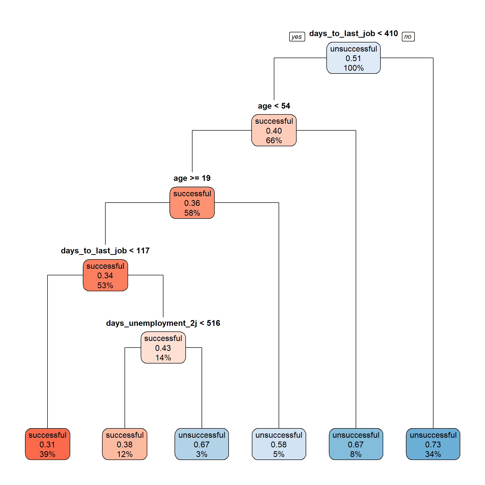
Confusion Matrix in R
Confusion Matrix and Statistics

              Reference
Prediction     successful unsuccessful
  successful          468          298
  unsuccessful        260          544

               Accuracy : 0.6446
                 95% CI : (0.6203, 0.6683)
    No Information Rate : 0.5363
    P-Value [Acc > NIR] : <2e-16

                  Kappa : 0.2879

 Mcnemar's Test P-Value : 0.1173

            Sensitivity : 0.6429
            Specificity : 0.6461
         Pos Pred Value : 0.6110
         Neg Pred Value : 0.6766
             Prevalence : 0.4637
         Detection Rate : 0.2981
   Detection Prevalence : 0.4879
      Balanced Accuracy : 0.6445

       'Positive' Class : successful
Cut-Off in R
test$score_tree <- predict(
  tree,
  newdata = test,
  type = c("prob")
  )[,1]

test <- test |>
  mutate(prediction_tree = as.factor(ifelse(
    score_tree > 0.3 ,
    "successful",
    "unsuccessful"
    )))

confusion <- confusionMatrix(
  data = test$prediction_tree,
  reference = test$target_low,
  positive = "successful",
  mode = "sens_spec"
  )
Confusion Matrix and Statistics
Reference
Prediction successful unsuccessful
successful 565 466
unsuccessful 163 376
Accuracy : 0.5994
95% CI : (0.5746, 0.6237)
No Information Rate : 0.5363
P-Value [Acc > NIR] : 2.776e-07
Kappa : 0.2166
Mcnemar's Test P-Value : < 2.2e-16
Sensitivity : 0.7761
Specificity : 0.4466
Pos Pred Value : 0.5480
Neg Pred Value : 0.6976
Prevalence : 0.4637
Detection Rate : 0.3599
Detection Prevalence : 0.6567
Balanced Accuracy : 0.6113
'Positive' Class : successful
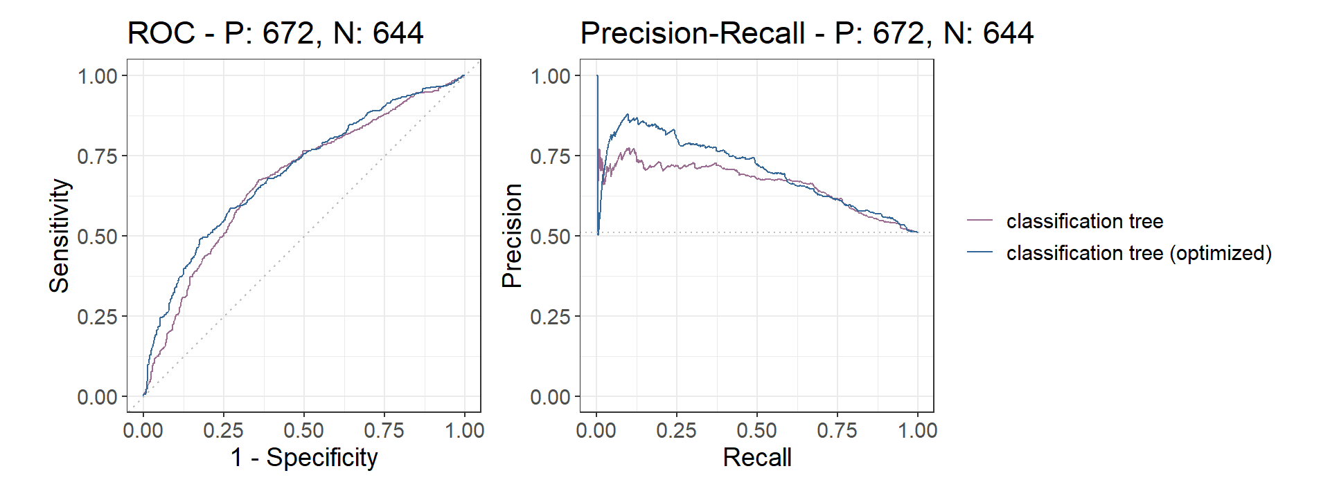
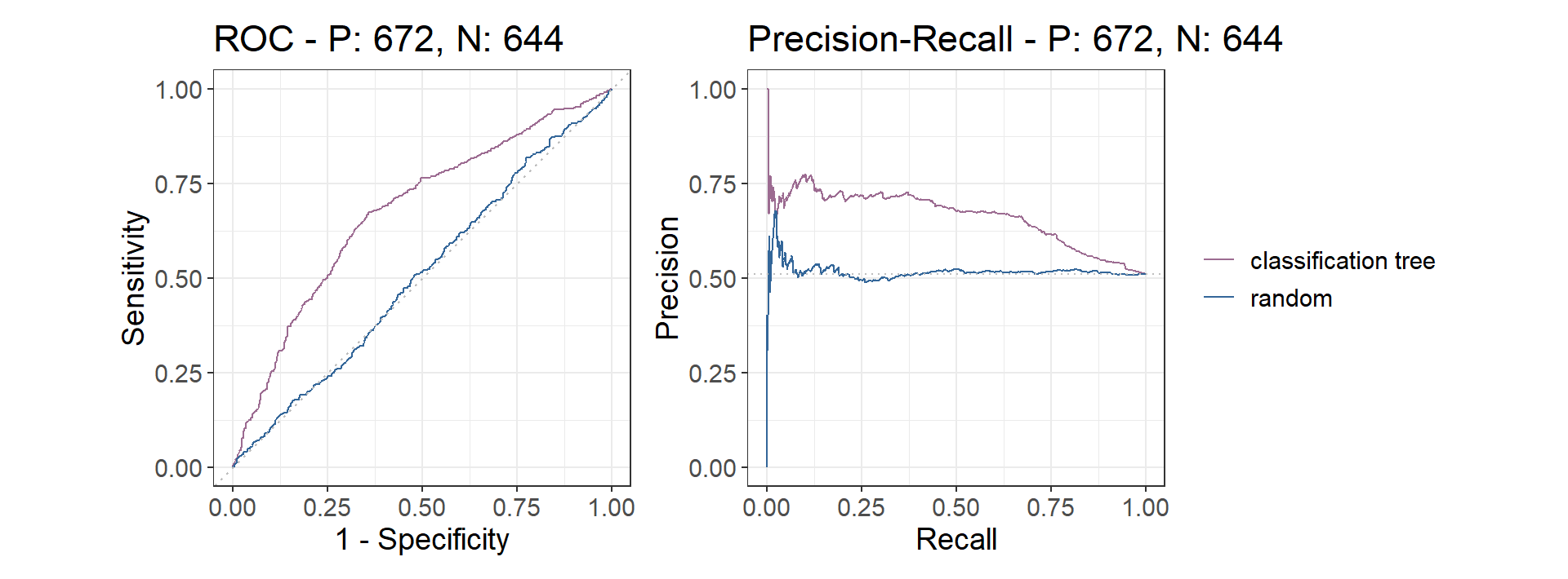
ROC- and PR-Curve in R
test$prediction_tree_scores <- predict(tree, test, type = c("prob"))[,2]
test$prediction_random <- runif(n = nrow(test))

precrec_obj <- evalmod(
  scores = cbind(test$prediction_tree_scores, test$prediction_random),
  labels = cbind(test$target_low, test$target_low),
  modnames = c("classification tree", "random"),
  ties_method = "first"
  )
CV in R - Caret
caret: classification and regression training
trControltakes care of the cross-validation processmethodhere specifies type of CVsummaryFunctionspecifies computation of performance measures
tuneGridchooses the parameters to try for the model
Training the Model
metricchooses what performance measure you want to optimizemethodspecifies the model, which can be implemented in some other package- Function will automatically choose the parameters which work best in the specified training and test process
CART

4830 samples
   3 predictor
   2 classes: 'successful', 'unsuccessful'

No pre-processing
Resampling: Cross-Validated (10 fold, repeated 10 times)
Summary of sample sizes: 4346, 4348, 4347, 4347, 4347, 4347, ...
Resampling results across tuning parameters:

  cp     ROC        Sens       Spec
  5e-04  0.7173981  0.6741891  0.6543656
  1e-03  0.7169620  0.7072193  0.6465661
  5e-03  0.6996839  0.6867633  0.6737720
  5e-02  0.6612506  0.7439858  0.5740977

ROC was used to select the optimal model using the largest value.
The final value used for the model was cp = 5e-04.
Extracting the Model
Predicting in Test Data
Confusion Matrix and Statistics

              Reference
Prediction     successful unsuccessful
  successful          409          235
  unsuccessful        234          438

               Accuracy : 0.6436
                 95% CI : (0.6171, 0.6695)
    No Information Rate : 0.5114
    P-Value [Acc > NIR] : <2e-16

                  Kappa : 0.2869

 Mcnemar's Test P-Value : 1

            Sensitivity : 0.6361
            Specificity : 0.6508
         Pos Pred Value : 0.6351
         Neg Pred Value : 0.6518
             Prevalence : 0.4886
         Detection Rate : 0.3108
   Detection Prevalence : 0.4894
      Balanced Accuracy : 0.6434

       'Positive' Class : successful
Model Comparison
test$prediction_caret_scores <- predict.train(
  tree_caret,
  test,
  type = c("prob"),
  na.action = na.pass
  )$unsuccessful

precrec_obj <- evalmod(
  scores = cbind(test$prediction_tree_scores, test$prediction_caret_scores),
  labels = cbind(test$target_low, test$target_low),
  modnames = c("classification tree", "classification tree (optimized)"),
  ties_method = "first"
  )