Introduction to Neural Networks

Data Science and Machine learning

Ines Kusmenko

Neural network jargon, that you will learn today…

perceptron
activation function
epoch
learning rate

gradient descent
backpropagation
hidden layers
deep learning

Introduction to Neural Networks

What is a Neural Network?

Neural networks are computational systems inspired by biological neural networks They can approximate non-linear relationships by learning from data.

They are composed of interconnected nodes (neurons) organized in layers.

Neural networks are particularly effective for:

Pattern recognition
Classification tasks
Regression problems

Applications: Remote Sensing and Image Recognition

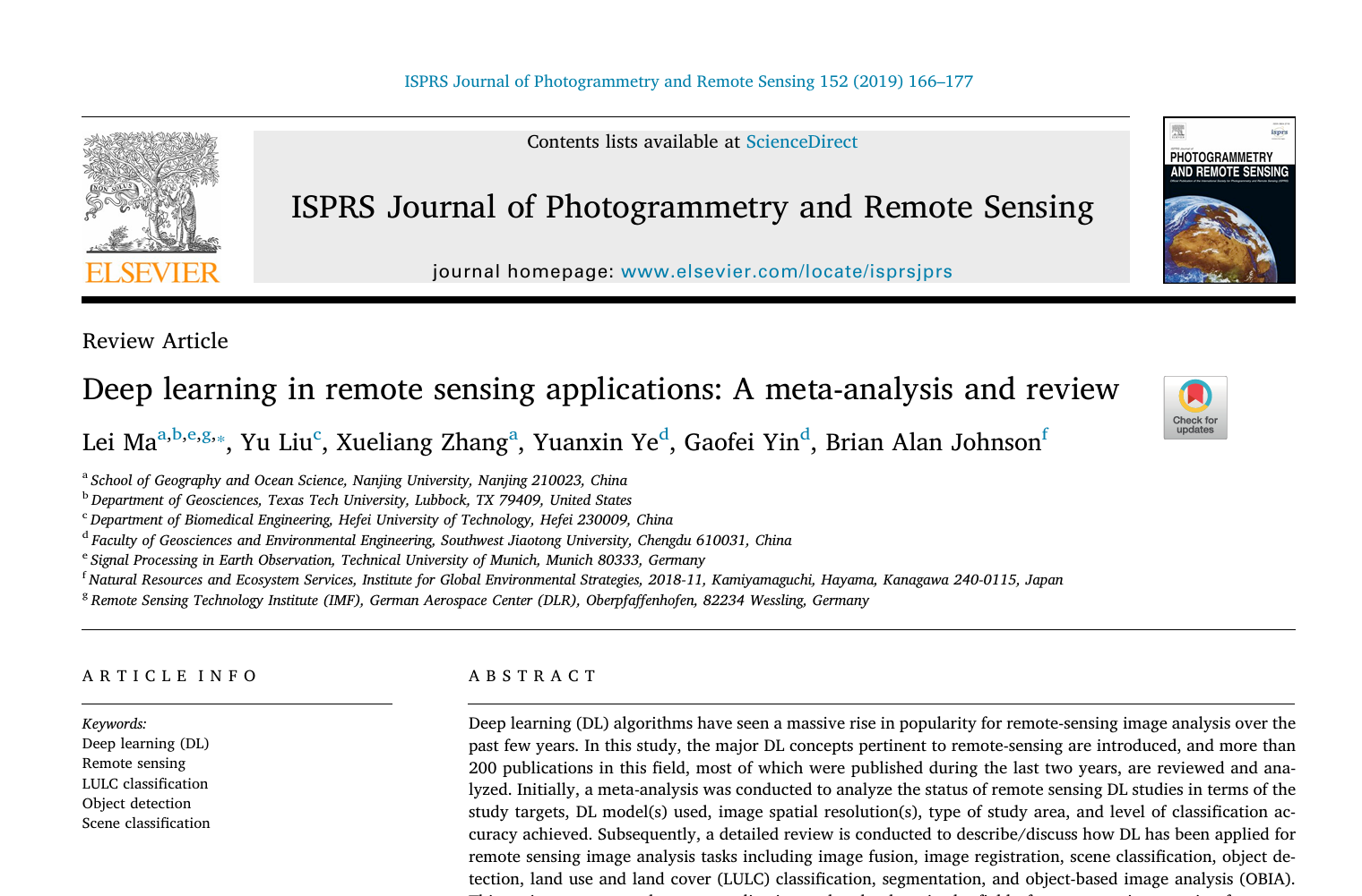
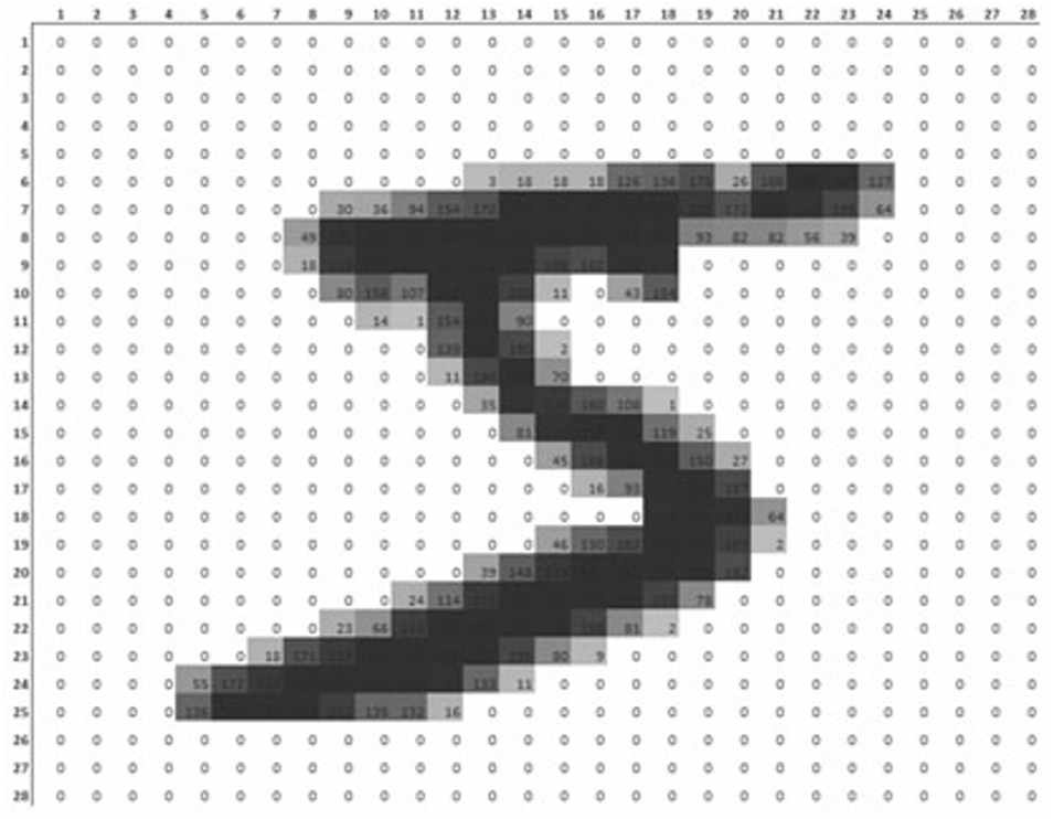
Applications: Image Recognition (I)

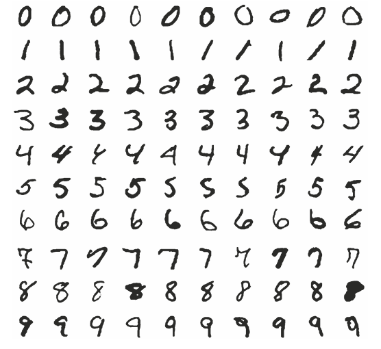
Applications: Image Recognition (II)

Applications: Macro (I)

Applications: Macro (II)

Applications (IV)

Econ Literature Pipeline

History (I)

McCulloch, W.S. and Pitts, W. (1943). A logical calculus of the ideas immanent in nervous activity. The bulletin of mathematical biophysics, 5(4):115–133.

History (II)

Rosenblatt, F. (1958). The perceptron: a probabilistic model for information storage and organization in the brain. Psychological review, 65(6), 386.

Main research questions:

How do (highly developed) organisms store information?
Does stored information influence the recognition of objects?

The biological neuron

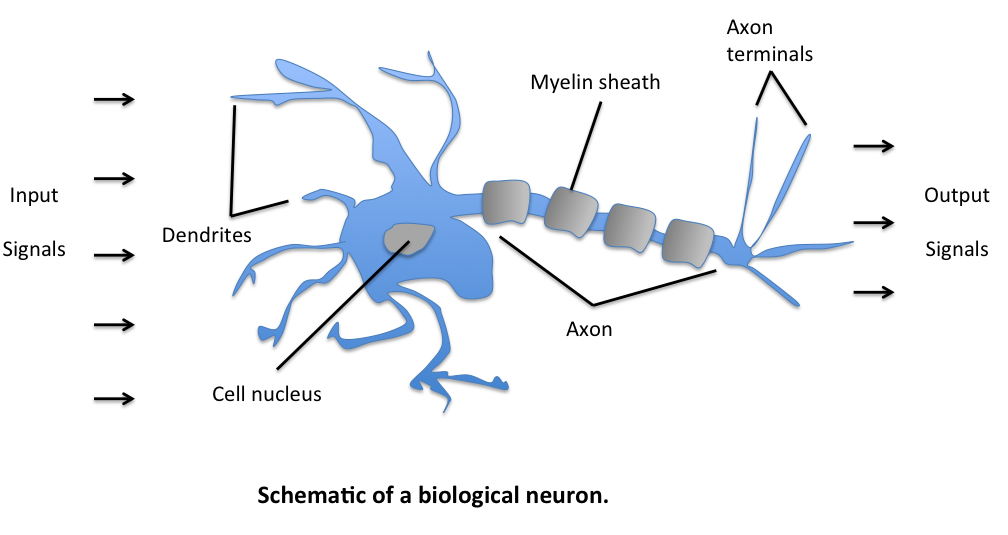
Schematic illustration of a biological neuron. Source: Sebastian Raschka.

Key insight: Learning occurs through strengthening or weakening synaptic connections

From neuron to perceptron

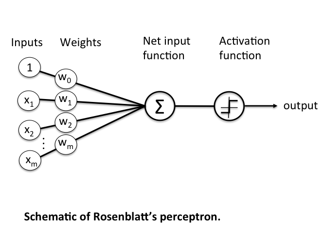
Illustration of a perceptron. Source: Sebastian Raschka.

The perceptron is a mathematical model inspired by biological neurons.

Perceptron decision rule: main formula

\[ z = \sum_{i=1}^{n} w_i x_i + b \]

\[ \text{Output} = f(z) = \begin{cases} 1, & \text{if } z > 0 \\ 0, & \text{otherwise} \end{cases} \]

Example 1: Simple perceptron calculation

Given:

$w_1 = 0.5, w_2 = -0.4$
$x_1 = 1, x_2 = 0$
$b = -0.3$

Calculation:

\[ z = (0.5 \times 1) + (-0.4 \times 0) + (-0.3) = 0.5 - 0.3 = 0.2 \]

Since $z = 0.2 > 0$, output = 1

Example 2: Another perceptron calculation

Given:

$w_1 = 0.3, w_2 = 0.7$
$x_1 = 1, x_2 = 1$
$b = -0.5$

Calculation:

\[ z = (0.3 \times 1) + (0.7 \times 1) + (-0.5) = 0.3 + 0.7 - 0.5 = 0.5 \]

Since $z = 0.5 > 0$, output = 1

Example 3: Perceptron outputs 0

Given:

$w_1 = 0.2, w_2 = 0.3$
$x_1 = 0$, $x_2 = 1$
Bias $b = -0.5$

\[ z = (0.2 \times 0) + (0.3 \times 1) + (-0.5) = 0.3 - 0.5 = -0.2 \]

Since $z = -0.2 < 0$, output = 0

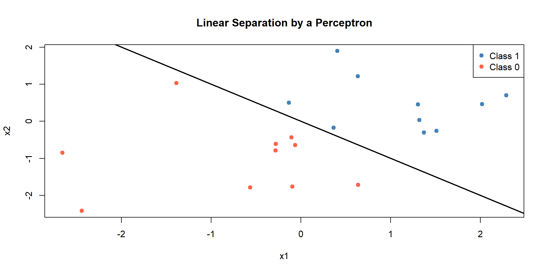
Example 1: Simple XOR Problem

XOR Problem

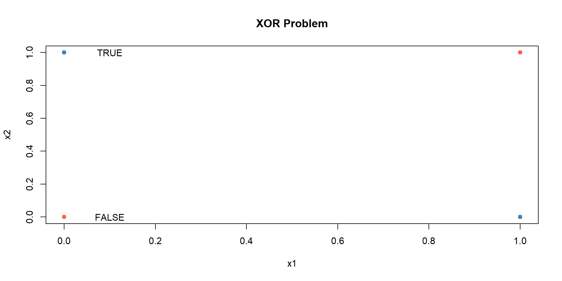
Non-linear classification with neural networks

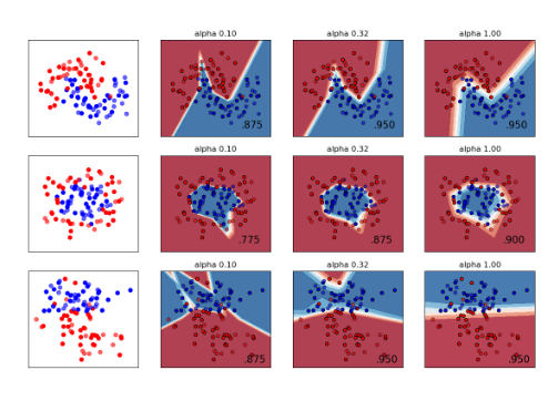
Neural Network Architecture

Basic Components of a Neural Network (I)

A single neuron performs:

\[z = \sum_{i=1}^{n} w_i x_i + b\]

Where:

$x_i$ = input values
$w_i$ = weights (connection strengths)
$b$ = bias term

Basic Components of a Neural Network (II)

\[y = f(z)\]

$f$ = activation function
$y$ = output

Activation Functions

Activation functions introduce non-linearity to the network.

Without activation functions, neural networks would be linear models
Activation functions enable networks to learn complex patterns

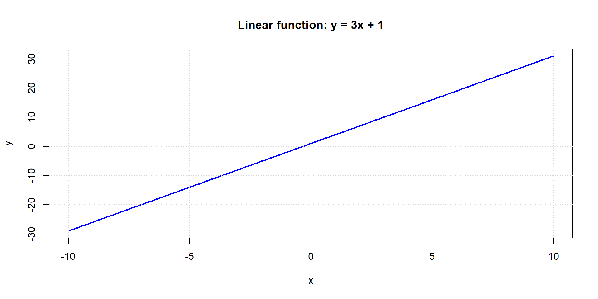
Linear function

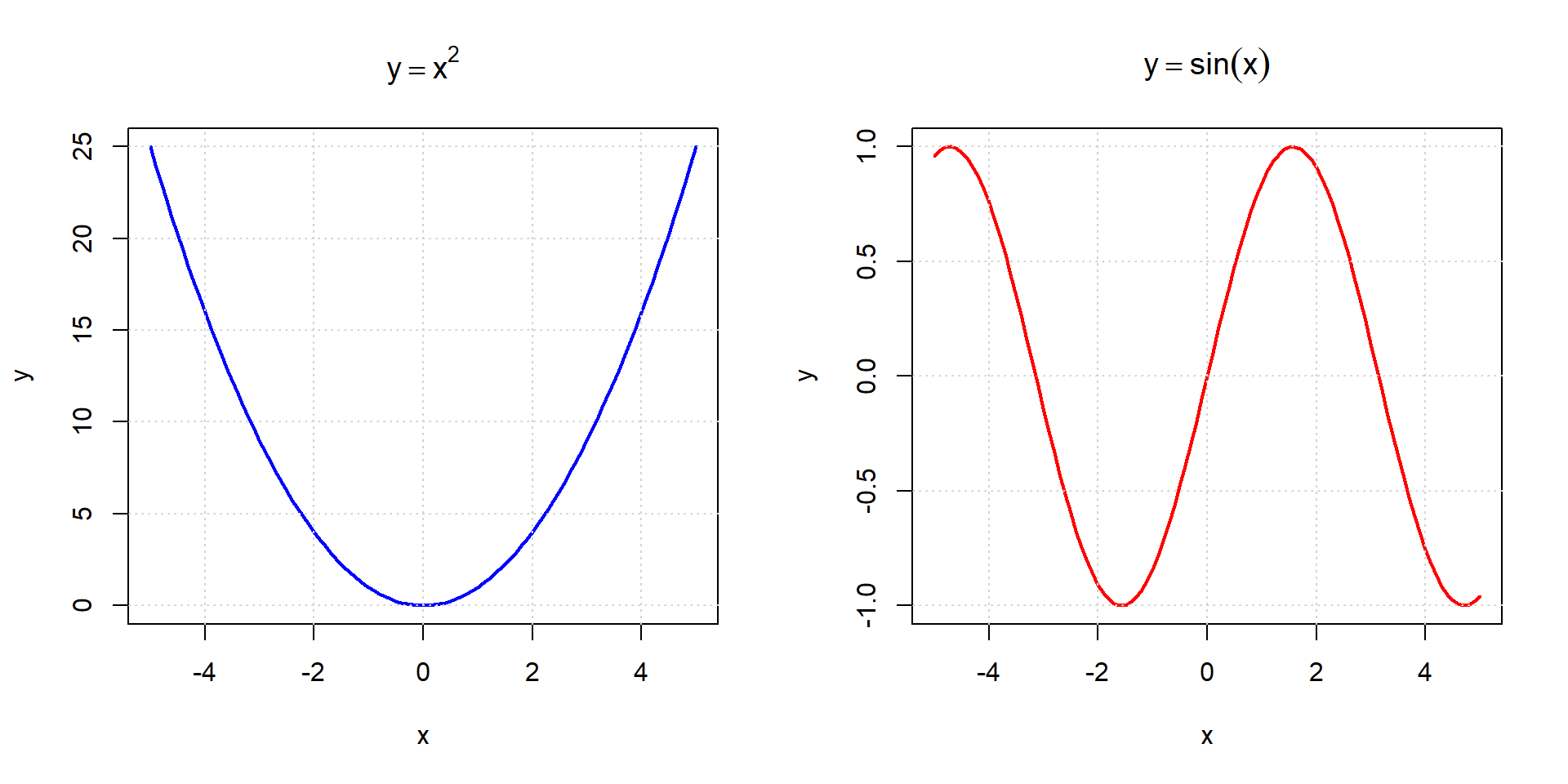
Higher degree / non-linear functions

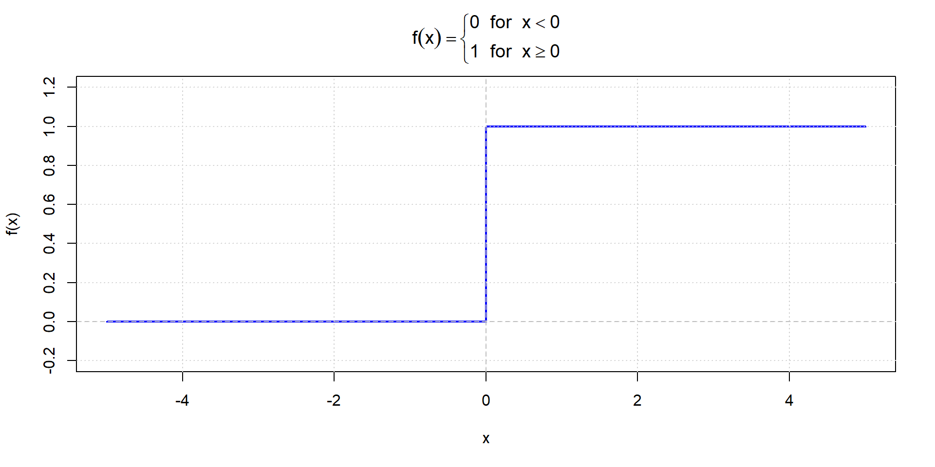
Step function

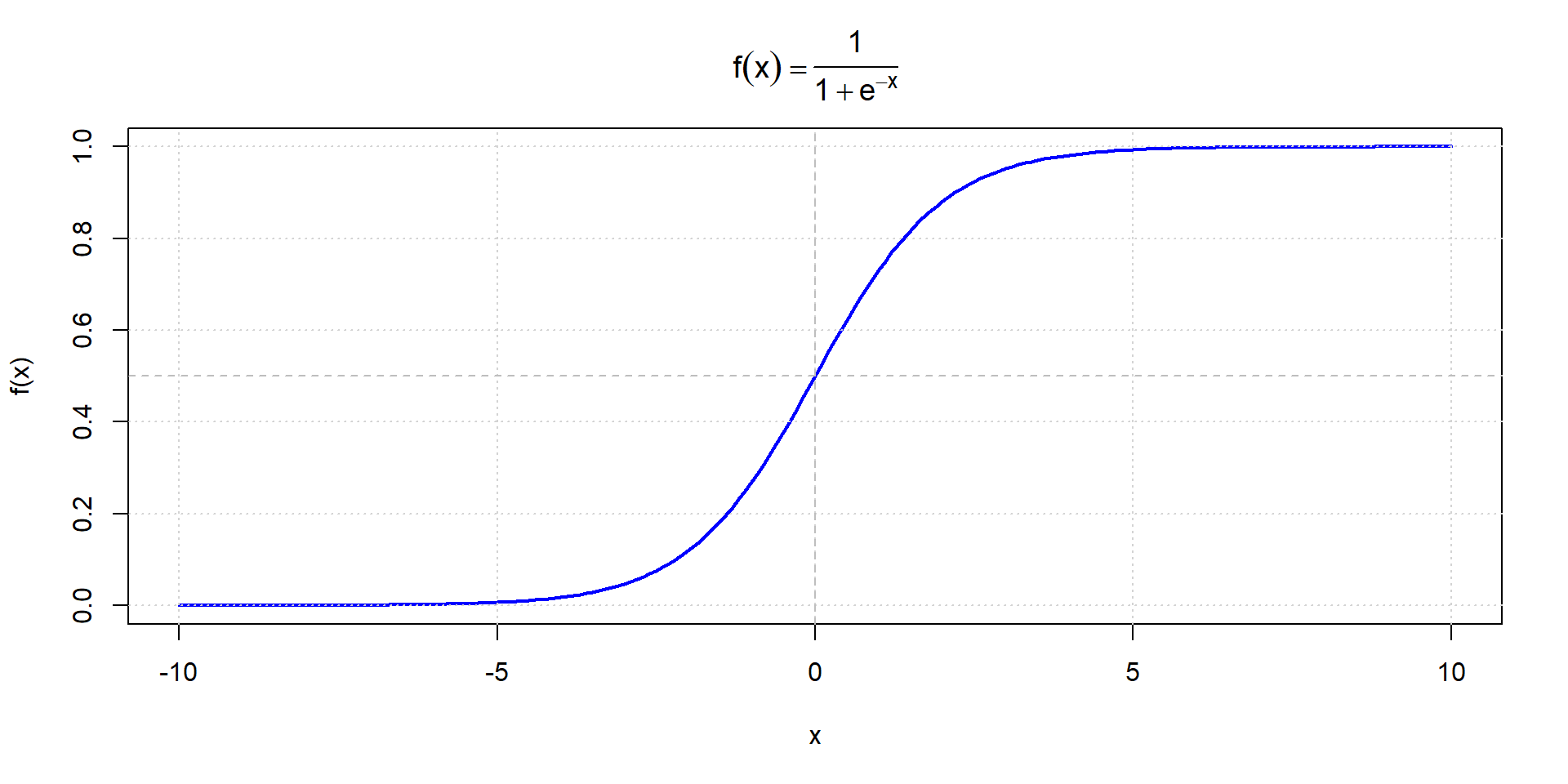
Sigmoid function

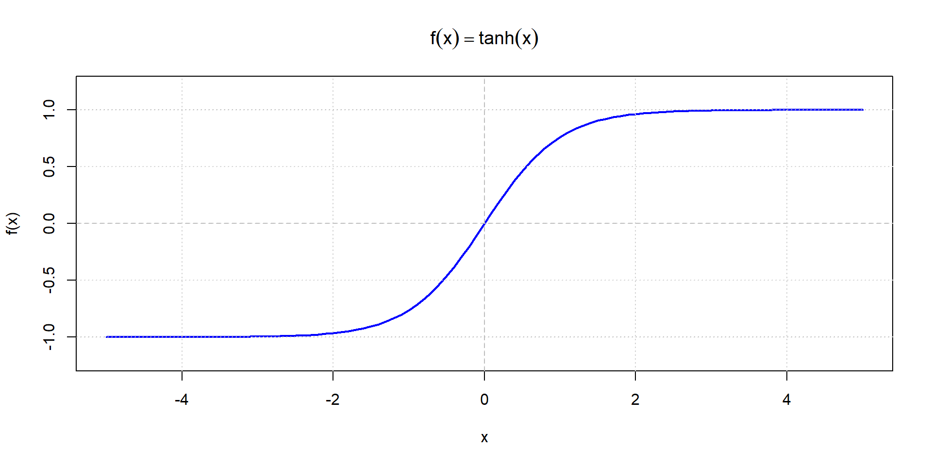
Hyperbolic tangent (tanh)

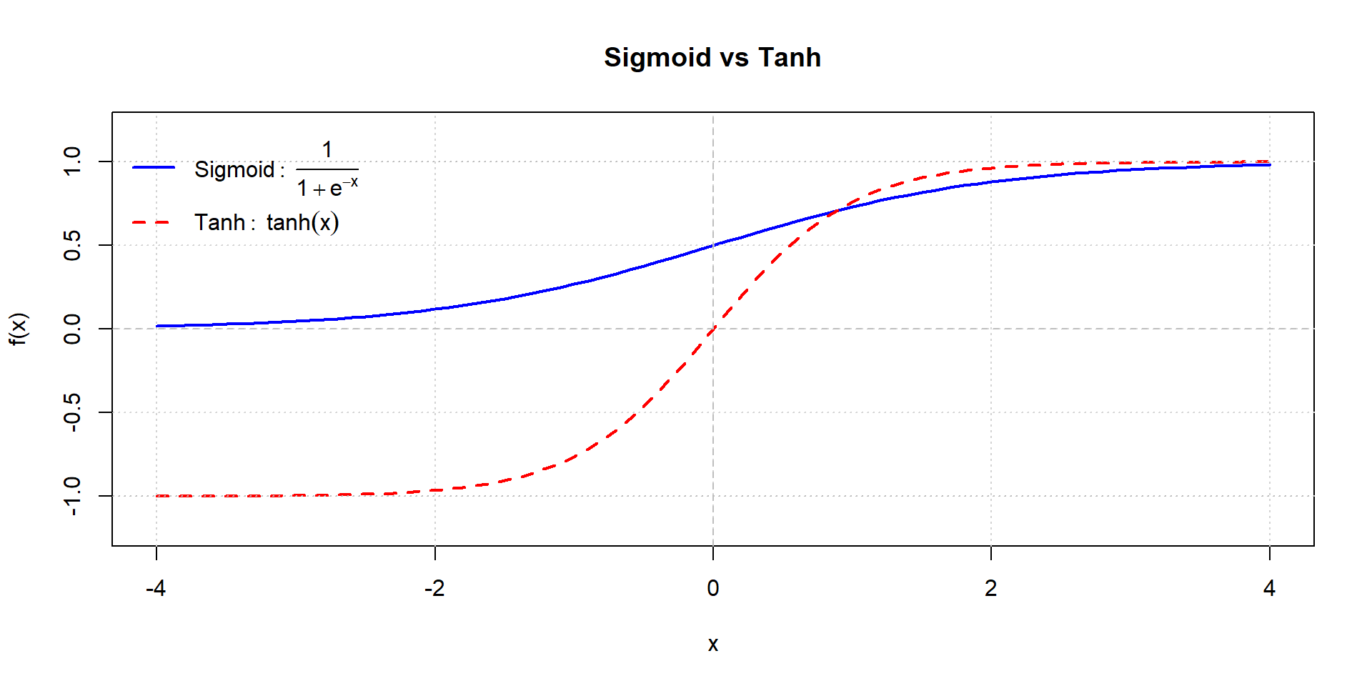
Sigmoid vs. tanh comparison

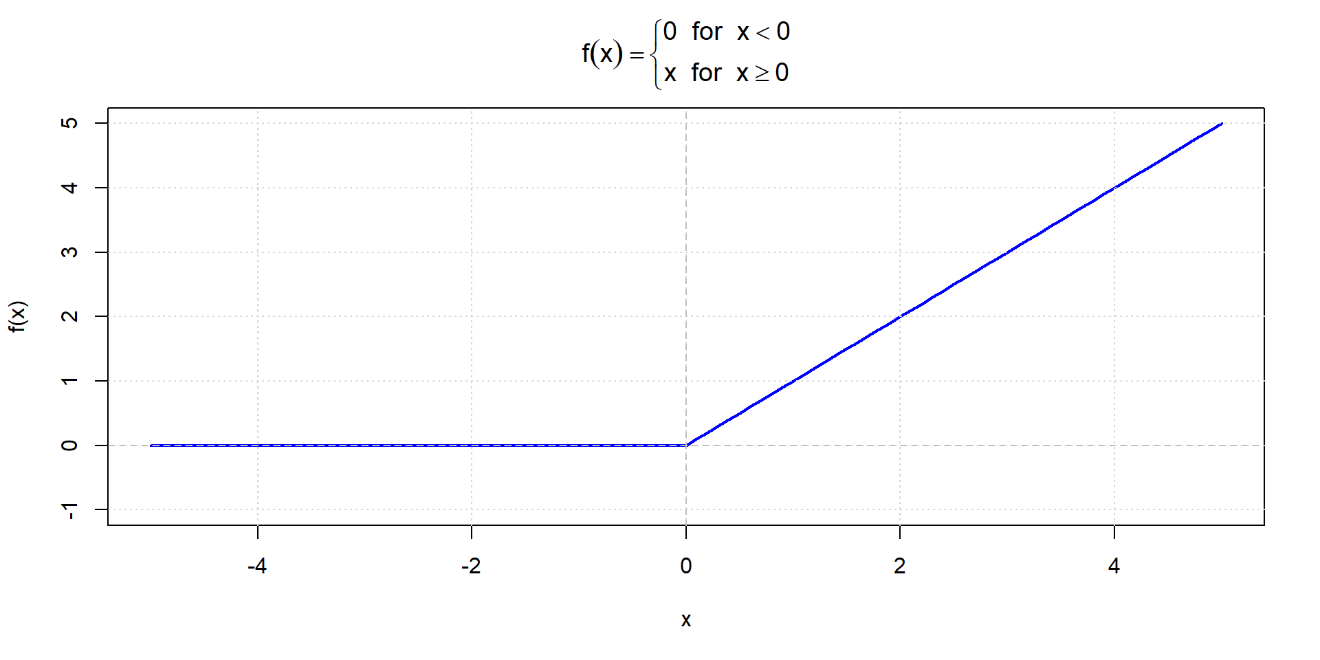
ReLU function

Training Neural Networks

What is Training

“Training is the act of presenting the network with some sample data and modifying the weights to better approximate the desired function”

The network learns by adjusting weights and biases
Goal: Minimize the difference between predicted and actual outputs

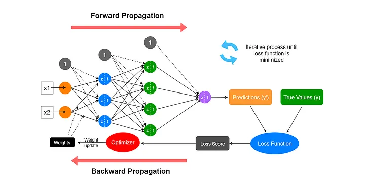
Forward Propagation and Backpropagation

Forward Propagation

Definition: Processing from input layer → hidden layer → output layer

The forward pass computes:

Weighted sum at each neuron: $z = wx + b$
Apply activation function: $a = f(z)$
Pass to next layer
Repeat until output layer
Calculate prediction

Forward Propagation Steps

For a network with one hidden layer:

Hidden Layer: \[z^{(1)} = w^{(1)}x + b^{(1)}\] \[a^{(1)} = f(z^{(1)})\]

Output Layer: \[z^{(2)} = w^{(2)}a^{(2)} + b^{(2)}\] \[\hat{y} = f(z^{(2)})\]

Computing the Error

At the output layer, we compute the error:

\[\text{Error} = \text{Predicted Output} - \text{Actual Output}\]

Backpropagation (I)

Definition: The process of propagating the error backward through the network to update weights

We correct the error in the process of backpropagation
Uses the partial derivative of each neuron’s activation function
The amount by which the weight should change is determined by gradient descent

Backpropagation (II)

backpropagation - schematic illustration. Source: Medium.com

The Training Algorithm (I)

Complete training process:

Take the matrix-based input
Assign initially random weights and biases
Apply inputs to the network
Calculate the output through the hidden layer(s) (forward propagation)

The Training Algorithm (II)

At the output layer: calculate the error
Compute error signals for previous layers using the partial derivative of the activation function (backpropagation)
Use the error signals to compute weight adjustments
Apply the weight adjustments
Repeat steps 3 to 8 until error is minimized

Gradient Descent

What is Gradient Descent?

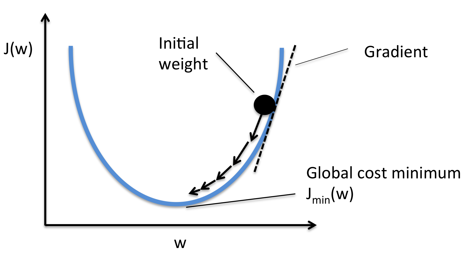
Optimization algorithm to minimize the loss function
Iteratively adjusts weights in the direction that reduces error

What is Gradient Descent?

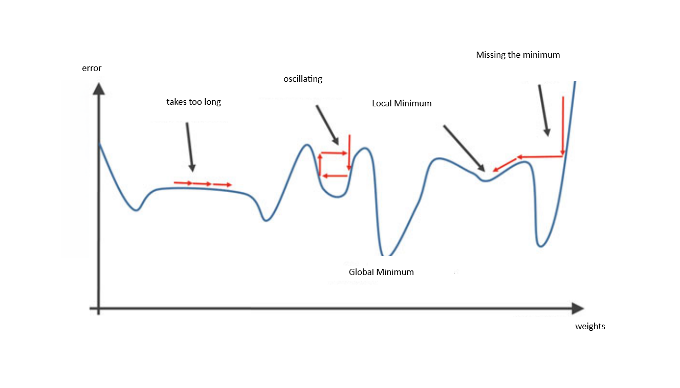
Potential errors in Backpropagation. Source: Sonnet (2022).

The Learning Rate

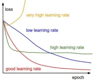
Learning rate - schematic illustration. Source: Medium.com

The learning rate is our step-size in adjusting weights:

New weight = Existing weight — Learning rate * Gradient

Gradient Descent explained

3Blue1Brown Video

“Gradient descent, how neural networks learn” Watch on YouTube

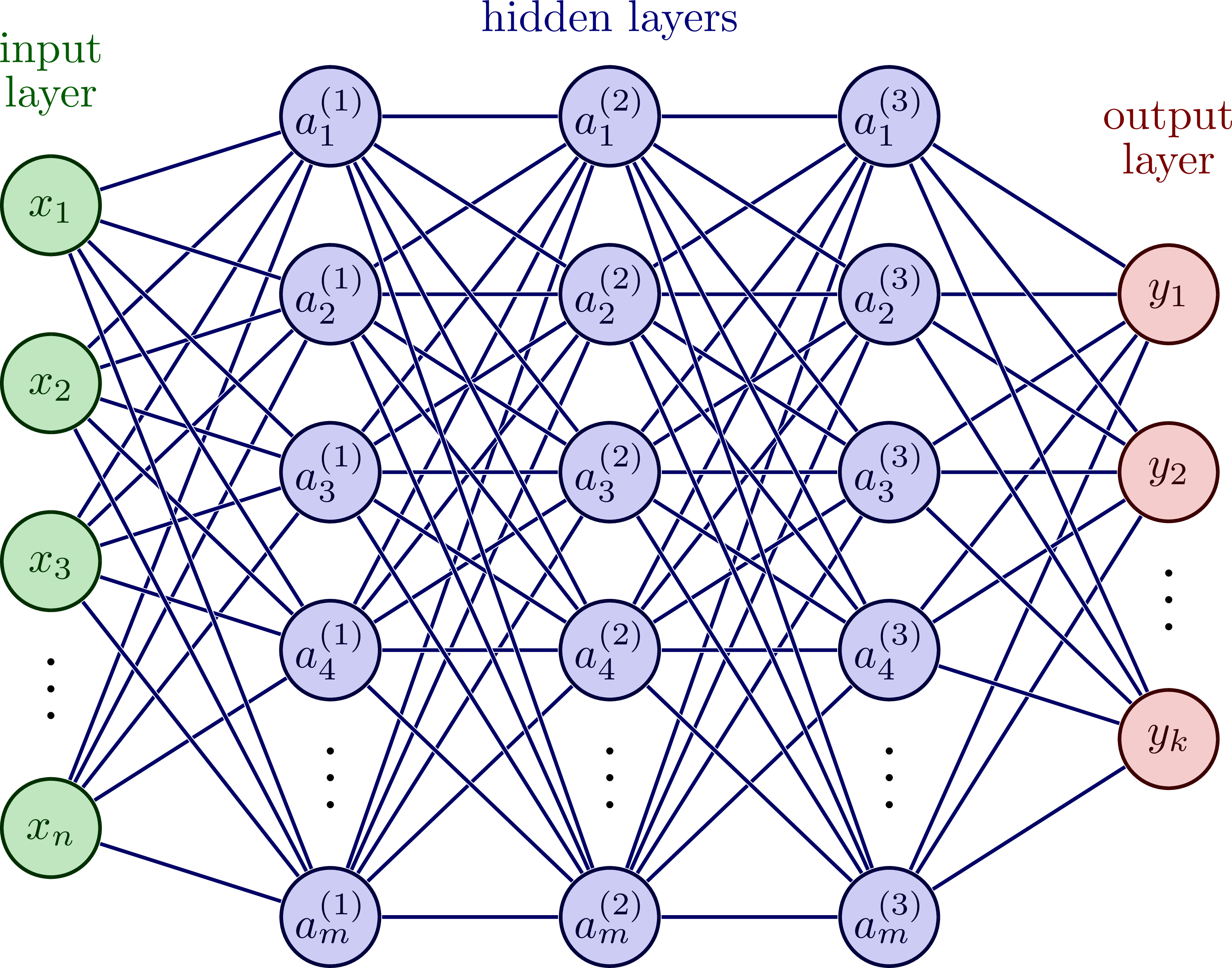
Multi-layer Neural Network Structure

Fully connected: each neuron connects to all neurons in next layer

Multiple Hidden Layers (Deep Learning)

Shallow networks: 1 hidden layer
Deep networks: 2+ hidden layers
Deeper networks can learn more complex patterns
Trade-offs:
- More expressive power
- Longer training time
- Requires more data

Types of Learning

Three main paradigms:

Supervised Learning
Unsupervised Learning
Reinforcement Learning

Supervised Learning

Training with labeled data (input-output pairs)
The network learns the mapping from inputs to outputs
Examples:
- Image classification (cat vs. dog)
- Spam detection
- House price prediction
Most common type for neural networks

Unsupervised Learning

Training with unlabeled data
The network discovers patterns and structures
Examples:
- Customer segmentation
- Anomaly detection
No predefined target values

Reinforcement Learning

Learning through trial and error
Agent receives rewards or penalties for actions
Goal: Maximize cumulative reward over time
Examples:
- Game playing
- Robotics

Some Training Concepts

Epoch

Definition: One complete pass through the entire training dataset

One iteration of providing input and updating network weights
Training typically requires multiple epochs
Each epoch:
- All training examples are seen once
- Weights are updated multiple times
- Model progressively improves

Epoch vs Batch vs Iteration

Batch: Subset of training data processed together
Iteration: One weight update (processing one batch)
Epoch: Complete pass through all data

Example with 1000 samples:

Batch size = 100 → 10 iterations per epoch

Batch size = 250 → 4 iterations per epoch

Choosing Number of Epochs

Too few epochs: Underfitting
Too many epochs: Overfitting

Scaling

Why Scale Your Data?

Neural networks require scaled input data:

Features often have different ranges (e.g., 0-1 vs 1000-10000)
Large values can dominate gradients
Leads to:
- Slow convergence
- Unstable training
- Poor performance

Scaling Methods

1. Min-Max Normalization (scales to 0-1):

\[x_{\text{norm}} = \frac{x - x_{\min}}{x_{\max} - x_{\min}}\]

2. Z-score Standardization (mean=0, std=1):

\[x_{\text{std}} = \frac{x - \mu}{\sigma}\]

Understanding the Neural Network

A Neural Network Playground

Example: Boston Dataset

The Boston Dataset (I)

The Boston data frame contains 506 rows and 14 columns of housing market data from the Boston area.

Prediction goal: medv is our response variable (= median value of owner-occupied homes in USD thousand). We fit a regression model to explain variation in owner-occupied home value.

Variable Descriptions

Left Column

crim: Per capita crime rate by town

zn: Proportion of residential land zoned for lots over 25,000 sq.ft.

indus: Proportion of non-retail business acres per town

chas: Charles River dummy variable (= 1 if tract bounds river; 0 otherwise)

nox: Nitrogen oxides concentration (parts per 10 million)

rad: Index of accessibility to radial highways

tax: Full-value property-tax rate per $10,000

Right Column

rm: Average number of rooms per dwelling

age: Proportion of owner-occupied units built prior to 1940

dis: Weighted mean of distances to five Boston employment centres

ptratio: Pupil-teacher ratio by town

black: $1000(B_k - 0.63)^2$ where $B_k$ is the proportion of blacks by town

lstat: Lower status of the population (percent)

medv: Median value of owner-occupied homes in $1,000s (TARGET)

The Boston Dataset (II)

#|echo: true

library("neuralnet")
library("MASS")
library("dplyr")
library("mlbench")
library(magrittr)
library(patchwork)
library(ggplot2)
library("reshape2")

set.seed("3456")

data = Boston 
head(data)

     crim zn indus chas   nox    rm  age    dis rad tax ptratio  black lstat
1 0.00632 18  2.31    0 0.538 6.575 65.2 4.0900   1 296    15.3 396.90  4.98
2 0.02731  0  7.07    0 0.469 6.421 78.9 4.9671   2 242    17.8 396.90  9.14
3 0.02729  0  7.07    0 0.469 7.185 61.1 4.9671   2 242    17.8 392.83  4.03
4 0.03237  0  2.18    0 0.458 6.998 45.8 6.0622   3 222    18.7 394.63  2.94
5 0.06905  0  2.18    0 0.458 7.147 54.2 6.0622   3 222    18.7 396.90  5.33
6 0.02985  0  2.18    0 0.458 6.430 58.7 6.0622   3 222    18.7 394.12  5.21
  medv
1 24.0
2 21.6
3 34.7
4 33.4
5 36.2
6 28.7

Scaling

We first scale the data:

\[x_{\text{scaled}} = \frac{x - x_{\min}}{x_{\max} - x_{\min}}\]

# Min max normalization - Rescaling 
summary(data)

      crim                zn             indus            chas        
 Min.   : 0.00632   Min.   :  0.00   Min.   : 0.46   Min.   :0.00000  
 1st Qu.: 0.08205   1st Qu.:  0.00   1st Qu.: 5.19   1st Qu.:0.00000  
 Median : 0.25651   Median :  0.00   Median : 9.69   Median :0.00000  
 Mean   : 3.61352   Mean   : 11.36   Mean   :11.14   Mean   :0.06917  
 3rd Qu.: 3.67708   3rd Qu.: 12.50   3rd Qu.:18.10   3rd Qu.:0.00000  
 Max.   :88.97620   Max.   :100.00   Max.   :27.74   Max.   :1.00000  
      nox               rm             age              dis        
 Min.   :0.3850   Min.   :3.561   Min.   :  2.90   Min.   : 1.130  
 1st Qu.:0.4490   1st Qu.:5.886   1st Qu.: 45.02   1st Qu.: 2.100  
 Median :0.5380   Median :6.208   Median : 77.50   Median : 3.207  
 Mean   :0.5547   Mean   :6.285   Mean   : 68.57   Mean   : 3.795  
 3rd Qu.:0.6240   3rd Qu.:6.623   3rd Qu.: 94.08   3rd Qu.: 5.188  
 Max.   :0.8710   Max.   :8.780   Max.   :100.00   Max.   :12.127  
      rad              tax           ptratio          black       
 Min.   : 1.000   Min.   :187.0   Min.   :12.60   Min.   :  0.32  
 1st Qu.: 4.000   1st Qu.:279.0   1st Qu.:17.40   1st Qu.:375.38  
 Median : 5.000   Median :330.0   Median :19.05   Median :391.44  
 Mean   : 9.549   Mean   :408.2   Mean   :18.46   Mean   :356.67  
 3rd Qu.:24.000   3rd Qu.:666.0   3rd Qu.:20.20   3rd Qu.:396.23  
 Max.   :24.000   Max.   :711.0   Max.   :22.00   Max.   :396.90  
     lstat            medv      
 Min.   : 1.73   Min.   : 5.00  
 1st Qu.: 6.95   1st Qu.:17.02  
 Median :11.36   Median :21.20  
 Mean   :12.65   Mean   :22.53  
 3rd Qu.:16.95   3rd Qu.:25.00  
 Max.   :37.97   Max.   :50.00

max_data <- apply(data, 2, max)
min_data <- apply(data, 2, min)
data_scaled <- as.data.frame(scale(data, center = min_data, scale = max_data - min_data))

Build the training dataset

split  <-  sample(1:nrow(data),round(0.75*nrow(data)))

train_data <- as.data.frame(data_scaled[split,])
test_data <- as.data.frame(data_scaled[-split, ])

nrow(test_data)

[1] 126

nrow(train_data)

[1] 380

summary(train_data)

      crim                 zn             indus              chas        
 Min.   :0.0000522   Min.   :0.0000   Min.   :0.01026   Min.   :0.00000  
 1st Qu.:0.0008616   1st Qu.:0.0000   1st Qu.:0.17815   1st Qu.:0.00000  
 Median :0.0033157   Median :0.0000   Median :0.34604   Median :0.00000  
 Mean   :0.0398760   Mean   :0.1092   Mean   :0.39591   Mean   :0.07105  
 3rd Qu.:0.0463340   3rd Qu.:0.1250   3rd Qu.:0.64663   3rd Qu.:0.00000  
 Max.   :0.8264345   Max.   :1.0000   Max.   :1.00000   Max.   :1.00000  
      nox               rm               age              dis        
 Min.   :0.0000   Min.   :0.05787   Min.   :0.0000   Min.   :0.0000  
 1st Qu.:0.1296   1st Qu.:0.44309   1st Qu.:0.4343   1st Qu.:0.0890  
 Median :0.3148   Median :0.50326   Median :0.7626   Median :0.1952  
 Mean   :0.3516   Mean   :0.51985   Mean   :0.6737   Mean   :0.2432  
 3rd Qu.:0.5062   3rd Qu.:0.58392   3rd Qu.:0.9323   3rd Qu.:0.3648  
 Max.   :1.0000   Max.   :1.00000   Max.   :1.0000   Max.   :0.8712  
      rad              tax              ptratio           black         
 Min.   :0.0000   Min.   :0.001908   Min.   :0.0000   Min.   :0.005547  
 1st Qu.:0.1304   1st Qu.:0.179389   1st Qu.:0.5106   1st Qu.:0.940932  
 Median :0.1739   Median :0.272901   Median :0.6809   Median :0.986321  
 Mean   :0.3926   Mean   :0.434281   Mean   :0.6259   Mean   :0.890165  
 3rd Qu.:1.0000   3rd Qu.:0.914122   3rd Qu.:0.8085   3rd Qu.:0.998260  
 Max.   :1.0000   Max.   :1.000000   Max.   :1.0000   Max.   :1.000000  
     lstat              medv       
 Min.   :0.02042   Min.   :0.0000  
 1st Qu.:0.15542   1st Qu.:0.2567  
 Median :0.27525   Median :0.3578  
 Mean   :0.30949   Mean   :0.3872  
 3rd Qu.:0.42557   3rd Qu.:0.4383  
 Max.   :1.00000   Max.   :1.0000

Set-up the neural net

n = names(data)
f = as.formula(paste("medv ~ ", paste(n[!n %in% "medv"], collapse = "+" 
                                      )))

net = neuralnet(f, data = train_data, hidden = c(5,3), linear.output = T)

Neural Net structure

Take predictions, report the error

# predict with neural net on test data
predict_net <-  predict(net, test_data[,1:13])
predict_net_unscaled <-  as.data.frame(predict_net * (max(data$medv)- min(data$medv)) + min (data$medv))

# compute RMSEs
rmse.net <- caret::RMSE(predict_net, test_data$medv)
print(paste("RMSE neural net:", rmse.net))

[1] "RMSE neural net: 0.0631425251809264"

test_unscaled <- as.data.frame((test_data$medv) * (max(data$medv)- min(data$medv)) + min (data$medv))
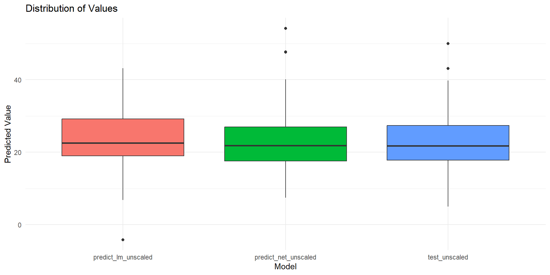
# Compare distribution of actual and predicted testing dataset 
summary(predict_net_unscaled)

       V1        
 Min.   : 7.443  
 1st Qu.:17.554  
 Median :21.831  
 Mean   :22.881  
 3rd Qu.:26.953  
 Max.   :54.213

summary(test_unscaled)

 (test_data$medv) * (max(data$medv) - min(data$medv)) + min(data$medv)
 Min.   : 5.00                                                        
 1st Qu.:17.80                                                        
 Median :21.80                                                        
 Mean   :22.85                                                        
 3rd Qu.:27.38                                                        
 Max.   :50.00

Regression model

Regression_Model <- glm(medv ~ ., data = train_data)
summary(Regression_Model)


Call:
glm(formula = medv ~ ., data = train_data)

Coefficients:
             Estimate Std. Error t value Pr(>|t|)    
(Intercept)  0.506041   0.064010   7.906 3.17e-14 ***
crim        -0.201157   0.090682  -2.218  0.02715 *  
zn           0.103714   0.037553   2.762  0.00604 ** 
indus       -0.012132   0.046426  -0.261  0.79399    
chas         0.070491   0.022767   3.096  0.00211 ** 
nox         -0.226284   0.049973  -4.528 8.06e-06 ***
rm           0.435719   0.058404   7.460 6.33e-13 ***
age         -0.005258   0.033573  -0.157  0.87564    
dis         -0.405556   0.059894  -6.771 5.10e-11 ***
rad          0.135291   0.042400   3.191  0.00154 ** 
tax         -0.107243   0.055410  -1.935  0.05370 .  
ptratio     -0.193583   0.033832  -5.722 2.19e-08 ***
black        0.087407   0.027217   3.211  0.00144 ** 
lstat       -0.420892   0.049694  -8.470 6.06e-16 ***
---
Signif. codes:  0 '***' 0.001 '**' 0.01 '*' 0.05 '.' 0.1 ' ' 1

(Dispersion parameter for gaussian family taken to be 0.01192427)

    Null deviance: 16.5010  on 379  degrees of freedom
Residual deviance:  4.3643  on 366  degrees of freedom
AIC: -588.96

Number of Fisher Scoring iterations: 2

Compare RMSE

predict_lm <- predict(Regression_Model, test_data[,1:13])
predict_lm_unscaled <-  as.data.frame(predict_lm * (max(data$medv)- min(data$medv)) + min (data$medv))

rmse.lm <- caret::RMSE(predict_lm, test_data$medv)
# Print the RMSE
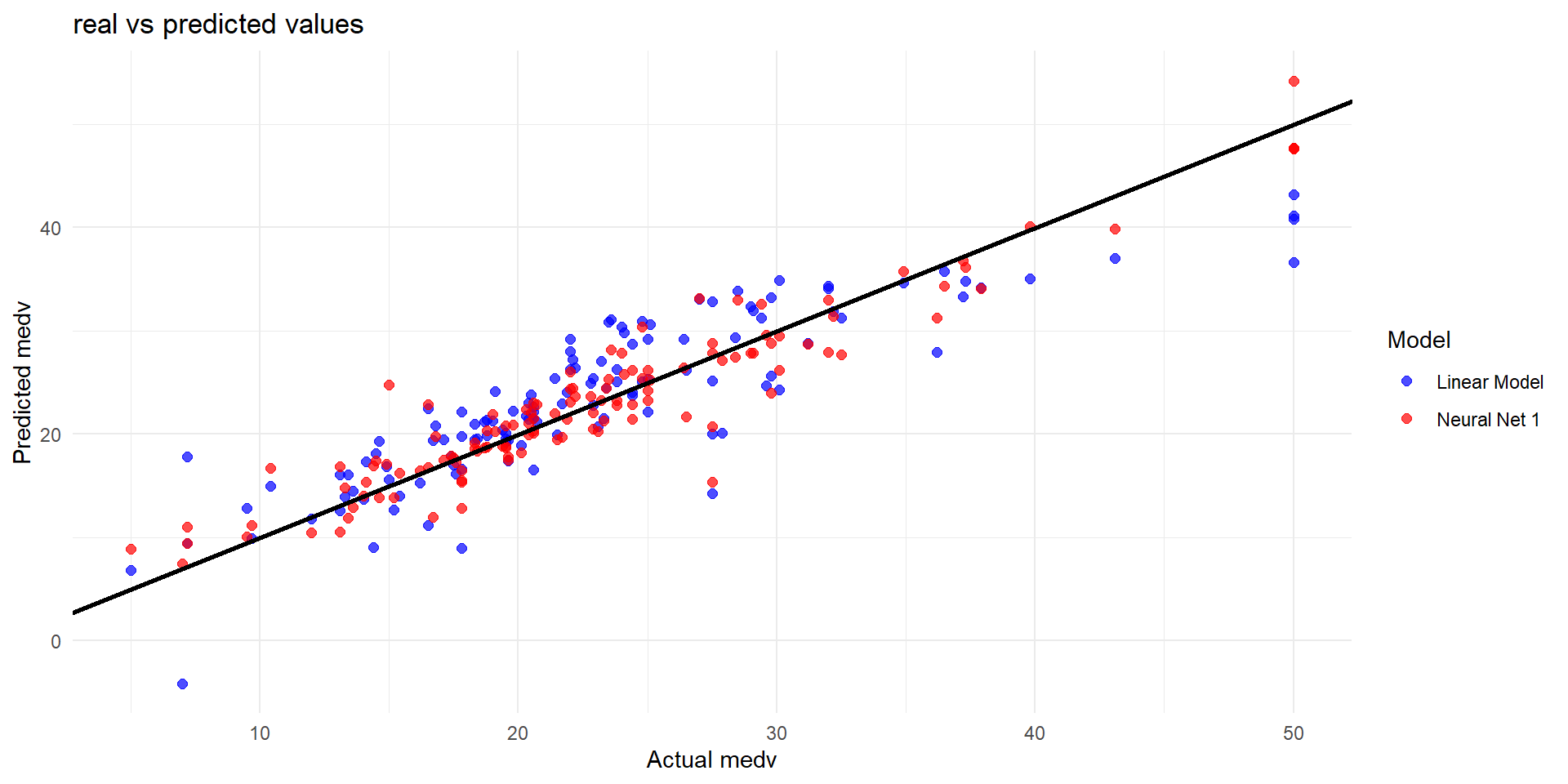
print(paste("Root Mean Squared Error Linear Model:", rmse.lm))

[1] "Root Mean Squared Error Linear Model: 0.0951616561991058"

# Print the RMSE
print(paste("Root Mean Squared Error Neural Net:", rmse.net))

[1] "Root Mean Squared Error Neural Net: 0.0631425251809264"

Plot actual predictions on tested data (I)

Plot actual predictions on tested data (II)

Key Takeaways

Neural networks learn by adjusting weights and biases
Forward propagation: Compute predictions
Backpropagation: Compute gradients and update weights
Gradient descent: Optimization algorithm
Epochs: Multiple passes through data needed
Data scaling: Essential preprocessing step
Three learning types: Supervised, Unsupervised, Reinforcement

Disadvantages of Neural Networks

NN are black-boxes
NN and other machine learning tools are estimators - they cannot replace causal identification
NN are computationally expensive and time-intensive
there is no specific rulebook on parameter settings
global vs local optimum

Assigment: Estimation exercise

Take a dataset of your choice and a dependent variable of interest
Explore the dataset: Set-up some descriptives (plot or table) for your variables
Set-up a prediction exercise:
- Choose a Machine Learning Tool of your choice and predict your dependent variable
- Based on the same data, use OLS
- Compare the results from OLS and your Machine Learning base estimator using RMSE or other performance criteria
- What of these performed better? What do you find more suitable for your data source?

References and further readings

Ciaburro, G., & Venkateswaran, B. (2017). Neural Networks with R. Packt Publishing.
Goodfellow, I., Bengio, Y., & Courville, A. (2016). Deep Learning. MIT Press.
3Blue1Brown. (2017). Neural Networks Series. YouTube.
Sonnet, D., Perceptron, V., & Learning, D. (2022). Neuronale Netze kompakt. IT kompakt. https://doi. org/10.1007/978-3-658-29081-8.
Zhang Z. Neural networks: further insights into error function, generalized weights and others. Ann Transl Med. 2016 Aug;4(16):300. doi: 10.21037/atm.2016.05.37. PMID: 27668220; PMCID: PMC5009026.