htl.html`
<div class="frame">
  <div class="table">
    <table width="1000px">
      <tr>
        <th></th>
        <th></th>
        <th colspan="2">Actual</th>
      </tr>
      <tr>
        <th></th>
        <th></th>
        <th>positive</th>
        <th>negative</th>
      </tr>
      <tr>
        <td rowspan="2" style="transform: rotate(-0deg);"><b>Predicted </b></td>
        <td><b>positive</b></td>
        <td style="background-color: rgba(45, 134, 89, 0.55);"># true positive (TP)</td>
        <td style="background-color: rgba(229, 35, 32, 0.55);"># false positive (FP)</td>
        <td><span class="formula">Precision = ${tex`\frac{TP}{TP+FP}`}</span></td>
      </tr>
      <tr>
        <td><b>negative</b></td>
        <td style="background-color: rgba(229, 35, 32, 0.55);"># false negative (FN)</td>
        <td style="background-color: rgba(45, 134, 89, 0.55);"># true negative (TN)</td>
        <td><span class="formula"> NPV = ${tex`\frac{TN}{TN+FN}`}</span></td>
      </tr>
      <tr>
        <td></td>
        <td></td>
        <td><span class="formula">Sensitivity = ${tex`\frac{TP}{TP+FN}`}</span></td>
        <td><span class="formula">Specificity = ${tex`\frac{TN}{TN+FP}`}</span></td>
        <td><span class="formula">Accuracy = ${tex`\frac{TP+TN}{n}`}</span></td>
      </tr>
    </table>
  </div>
</div>
`Confusion Matrix & Cross Validation
What even is a well performing model?
Confusion Matrix
Judging a classifier’s performance
Confusion Matrix
- for a classification problem we can look at a confusion matrix
Base-Rate Fallacy
- Beware of the base rate fallacy:
- Let’s assume the Austrian population is getting tested for the Coronavirus
- 1% of the population is indeed infected, meaning \(P(C) = 0.01\)
- A test is 98% accurate, in the sense that \(P(\text{Test}_C \mid C) = P(\text{Test}_{\neg C} \mid \neg C) = 0.98\)
- What is the probability that I have the Coronavirus given that I tested positive? \(P(C \mid \text{Test}_C)\)?
- Which value from the confusion matrix did we calculate here (and which ones were given)?
Judging Performance in Classification Problems
- All the indicators in the confusion matrix can be relevant
- Accuracy depends on base rate
- accuracy of 96% in sample with 95% positives → poor performance
- accuracy of 80% in sample with 50% positives → good performance
- Need for adjustment of values relative to a “naive prediction”
- Concepts can be generalized to classification problems with more than two categories
Adjusted Performance Measures
- Cohen’s kappa: \[ \kappa = \frac{Acc_{mod} - Acc_{0}}{1 - Acc_{0}} \] where \(Acc_{mod}\) is the accuracy of our model and \(Acc_{0}\) is the expected random accuracy
For any sensible model, it holds that \(0 < \kappa < 1\)
If \(\kappa < 0\), our model would be worse than guessing at random
\(\kappa\) tells you “how far you are away from predicting perfectly compared to a naive prediction”
ROC- and PR-Curve
- Trade-off between the measures, which we can exploit by setting the cut-off point for predicted scores
- Receiver Operating Characteristic (ROC) curve
- Plot of sensitivity against 1-specificity
- Helps identify which cut-off point to choose
- Precision-Recall (PR) curve
- Plot of precision against sensitivity (recall)
- Might be preferred over ROC when categories are very imbalanced
Receiver Operating Characteristic
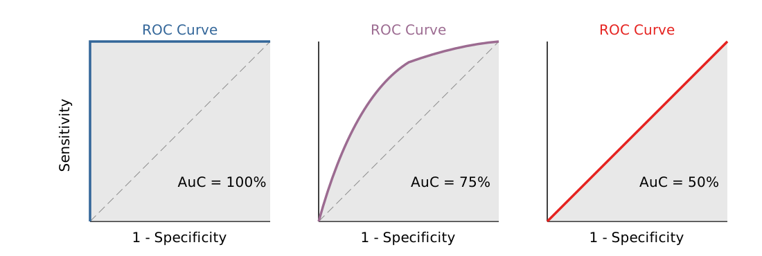
- The trade-off through the setting of the cut-off point can be visualized in a ROC curve
Receiver Operating Characteristic
- ROC criterion
- There is a point on the curve where the loss of sensitivity and specificity are equal
- This value can be used to determine an “optimal” cut-off point
- Sometimes high sensitivity is preferred over specificity (e.g., medical tests), or vice versa
- Area Under the Curve (AUC)
- The area underneath the ROC curve can be used as another performance measure
- Different models achieve different sensitivity and specificity at the same cut-off point
- The model with the highest AUC is best at holding the trade-off low
Interacting with the Cut-Off
import {Plot} from "@mkfreeman/plot-tooltip"
import {aq, op} from '@uwdata/arquero'

data = FileAttachment("data/cutOffData.csv").csv({ typed: true })

vizData = aq.from(data)
  .derive({
    score: aq.escape(d =>
      radios === "Balanced Good" ? d.target_low_score * 100 :
      radios === "Unbalanced Good" ? d.target_high_score * 100 :
      radios === "Balanced Mediocre" ? d.target_low_score_bad * 100 :
      d.target_high_score_bad * 100
    ),
    class: aq.escape(d =>
      radios === "Balanced Good" ? d.target_low :
      radios === "Unbalanced Good" ? d.target_high :
      radios === "Balanced Mediocre" ? d.target_low :
      d.target_high
    ),
  })
  .derive({
    classPredicted: aq.escape(d => d.score > range ? "successful" : "unsuccessful"),
  })
  .derive({
    type: d =>
      d.class === "successful" && d.classPredicted === "successful" ? "TP" :
      d.class === "unsuccessful" && d.classPredicted === "successful" ? "FP" :
      d.class === "unsuccessful" && d.classPredicted === "unsuccessful" ? "TN" :
      d.class === "successful" && d.classPredicted === "unsuccessful" ? "FN": null,
  })

fullType = aq.from([
  {type: "TP"},
  {type: "FP"},
  {type: "FN"},
  {type: "TN"},
])

FP = values.filter(d => d.type === "FP").map(d => d.count)[0]
TP = values.filter(d => d.type === "TP").map(d => d.count)[0]
FN = values.filter(d => d.type === "FN").map(d => d.count)[0]
TN = values.filter(d => d.type === "TN").map(d => d.count)[0]

values = vizData
  .groupby("type")
  .rollup({
    count: d => op.count(),
  })
  .join_full(fullType, "type")
  .derive({
    count: d => d.count === undefined ? 0 : d.count,
  })
  .orderby("type")
  .objects()

cutOffs = aq.table({ cutOff: Array.from(Array(101).keys()) })
  .derive({
    identity: aq.escape(d => "1"),
  })

CutOffData = aq.from(data)
  .derive({
    score: aq.escape(d =>
      radios === "Balanced Good" ? d.target_low_score * 100 :
      radios === "Unbalanced Good" ? d.target_high_score * 100 :
      radios === "Balanced Mediocre" ? d.target_low_score_bad * 100 :
      d.target_high_score_bad * 100
    ),
    class: aq.escape(d =>
      radios === "Balanced Good" ? d.target_low :
      radios === "Unbalanced Good" ? d.target_high :
      radios === "Balanced Mediocre" ? d.target_low :
      d.target_high
    ),
  })
  .derive({
    identity: aq.escape(d => "1"),
  })
  .join_full(cutOffs, "identity")
  .derive({
    classPredicted: aq.escape(d => d.score > d.cutOff ? "successful" : "unsuccessful"),
  })
  .derive({
    type: d =>
      d.class === "successful" && d.classPredicted === "successful" ? "TP" :
      d.class === "unsuccessful" && d.classPredicted === "successful" ? "FP" :
      d.class === "unsuccessful" && d.classPredicted === "unsuccessful" ? "TN" :
      d.class === "successful" && d.classPredicted === "unsuccessful" ? "FN": null,
  })
  .groupby(["type", "cutOff"])
  .rollup({
    count: d => op.count(),
  })
  .join_full(fullType, "type")
  .derive({
    count: d => d.count === undefined ? 0 : d.count,
  })
  .orderby(["type", "cutOff"])
  .groupby("cutOff")
  .pivot("type", "count" ) // { count: d => d.count === undefined ? 0 : d.count}
  .derive({
    TN: d => d.TN === undefined ? 0 : d.TN,
    TP: d => d.TP === undefined ? 0 : d.TP,
    FN: d => d.FN === undefined ? 0 : d.FN,
    FP: d => d.FP === undefined ? 0 : d.FP,
  })
  .derive({
    Sensitivity: d => d.TP/(d.TP+d.FN)*100,
    "1-Specificity": d => 100 - d.TN/(d.TN+d.FP)*100,
    Precision: d => d.TP/(d.TP+d.FP)*100,
  })

numberOfObservations = vizData.rollup({n: d => op.count()}).objects().map(d => d.n)[0]

noInformationRate = Math.min(
  ... vizData
    .groupby("class")
    .rollup({
      noInformationRate: d => op.count()
    })
    .objects()
    .map(d => d.noInformationRate)
  ) /
  numberOfObservations * 100

PR = ({
  // title: "Precision-Recall",
  fontFamily: "Roboto",
  style: {fontSize: "11px"},
  width: 200,
  height: 200,
  marks: [
    Plot.ruleY([0]),
    Plot.lineY(CutOffData, {y: "Precision", x: "Sensitivity"}),
    Plot.dot([1], {y: TP/(TP+FP) * 100, x: TP/(TP+FN)*100, fill: "#e52320", r: 5, }),
    Plot.line([{x: 0, y: noInformationRate}, {x: 100, y: noInformationRate}], {stroke: "black", x: "x", y: "y", strokeDasharray: 4}),
    Plot.axisX({labelOffset: -10, label: "Sensitivity (Recall)"}),
    Plot.axisY({labelOffset: -10, label: "Precision"})
  ]
})

ROC = ({
  // title: "Receiver Operating Characteristic",
  fontFamily: "Roboto",
  style: {fontSize: "11px"},
  width: 200,
  height: 200,
  marks: [
    Plot.ruleY([0]),
    Plot.lineY(CutOffData, {x: "1-Specificity", y: "Sensitivity" , }),
    // Plot.areaY(CutOffData.orderby("Sensitivity"), {y: "Sensitivity", fillOpacity: 0.3}),
    Plot.dot([1], {x: (100 - TN/(TN+FP) * 100), y: TP/(TP+FN)*100, fill: "#e52320", r: 5, }),
    Plot.line([{x: 0, y: 0}, {x: 100, y: 100}], {stroke: "black", x: "x", y: "y", strokeDasharray: 4}),
    Plot.axisX({labelOffset: -10, label: "1-Specificity"}),
    Plot.axisY({labelOffset: -10, label: "Sensitivity"})
  ]
})

radius = 6

view = ({
  // title: "Distribution of Scores",
  fontFamily: "Century Gothic",
  style: { fontSize: "11px", backgroundColor: "transparent" },
  height: 480,
  width: 545,
  x: {domain: [0, 100]},
  color: {
    range: ["#e52320", "#e52320", "#2d8659", "#2d8659"],
    legend: false,
    columns: 2,
  },
  symbol: {
    legend: false,
    range: ["circle", "square"]
  },
  marks: [
    Plot.dot(
      vizData.join_full(fullType, "type"),
      Plot.dodgeY({
        x: "score",
        fill: "type",
        fillOpacity: 0.55,
        anchor: "bottom",
        r: radius,
        title: d => `${d.type}`,
        stroke: "black",
        strokeWidth: 1,
        symbol: "class",
      })
    ),
  Plot.ruleX([range], {strokeWidth: 2}),
  // Plot.text(
  //   values[0],
  //   {x: range, y: 10, text: "Hello"}
  //   ),
  Plot.area(
    {x1: 0, x2: range, y1: 0, y2: 100, fill: "#e52320", opacity: 0.5, }
  ),
  Plot.text(
      vizData.join_full(fullType, "type"),
      Plot.dodgeY({
        x: "score",
        fill: "type",
        r: radius,
        anchor: "bottom",
        text: "type",
        stroke: "black",
        fill: "black",
        strokeWidth: 0.1,
        fontSize: radius - 1,
        pointerEvents: "none"
      })
    ),
    Plot.axisX({anchor: "bottom", labelOffset: -10}),
  ],
  tooltip: {
    opacity: 0.5,
    stroke: "transparent"
  },
})
viewof radios = Inputs.radio(["Balanced Good", "Unbalanced Good", "Balanced Mediocre", "Unbalanced Mediocre"], {label: null, value: "Balanced Good"})
viewof range = Inputs.range([-1, 101], {label: null, step: 1, width: 440, value: 50, format: x => Math.round(x)})htl.html`
<div class="containerMatrix">
<div class="left-column">
${viewof radios}
<div class="left-row">
<table>
<tr>
<th></th>
<th></th>
<th colspan="2">Actual</th>
</tr>
<tr>
<th></th>
<th></th>
<th>positive</th>
<th>negative</th>
</tr>
<tr>
<td rowspan="2" style="transform: rotate(-0deg);"><b>Predicted </b></td>
<td><b>positive</b></td>
<td style="background-color: rgba(45, 134, 89, 0.55);">TP: ${TP}</td>
<td style="background-color: rgba(229, 35, 32, 0.55);">FP: ${FP}</td>
<td><span class="formula">Precision = ${Math.round(TP/(TP+FP) * 100) + "%"}</span></td>
</tr>
<tr>
<td><b>negative</b></td>
<td style="background-color: rgba(229, 35, 32, 0.55);">FN: ${FN}</td>
<td style="background-color: rgba(45, 134, 89, 0.55);">TN: ${TN}</td>
<td><span class="formula"> NPV = ${Math.round(TN/(TN+FN)*100) + "%"}</span></td>
</tr>
<tr>
<td></td>
<td></td>
<td><span class="formula">Sensitivity = ${Math.round(TP/(TP+FN)*100) + "%"}</span></td>
<td><span class="formula">Specificity = ${Math.round(TN/(TN+FP)*100) + "%"}</span></td>
<td><span class="formula">Accuracy = ${Math.round((TN + TP)/(TN+FP+FN+TP)*100) + "%"}</span></td>
</tr>
</table>
</div>
<div class="left-row left-row-2">
<div>
${Plot.plot(ROC)}
</div>
<div>
${Plot.plot(PR)}
</div>
</div>
</div>
<div class="right-column">
${Plot.plot(view)}
${viewof range}
</div>
</div>
`The Infamous “AMS-Algorithmus” I
- The AMAS has been criticized for intransparency (among other things)
- One of the few publicly available documents states the usage of a logit model (which was, contrary to public belief, never implemented) for this algorithm
- Or rather, two logit models:
- One predicting your short-term chance of labor market integration (assignment to group A if chances are high)
- One predicting your long-term labor market integration (assignment to group C if chances are low), given a set of demographic variables and your labor market history
- The assignment to groups A, B, and C determines if you are eligible for certain types of subsidies
The Infamous “AMS-Algorithmus” II
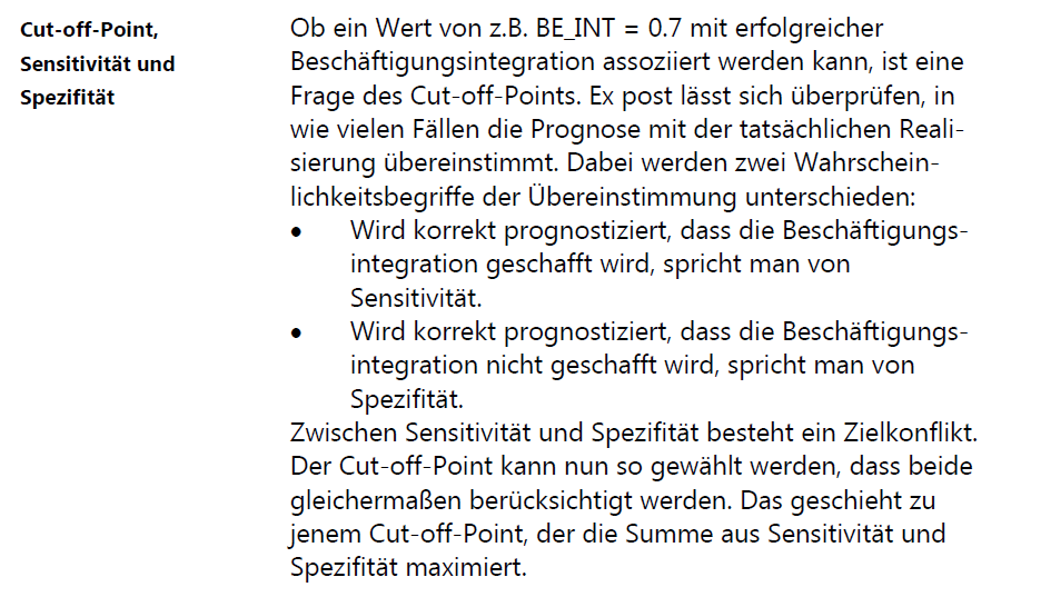
- In the documentation, it is correctly stated that the cut-off point can be chosen in a way to balance sensitivity and specificity (ignoring the strange definitions of Sensitivity and Specificity)
The Infamous “AMS-Algorithmus” III
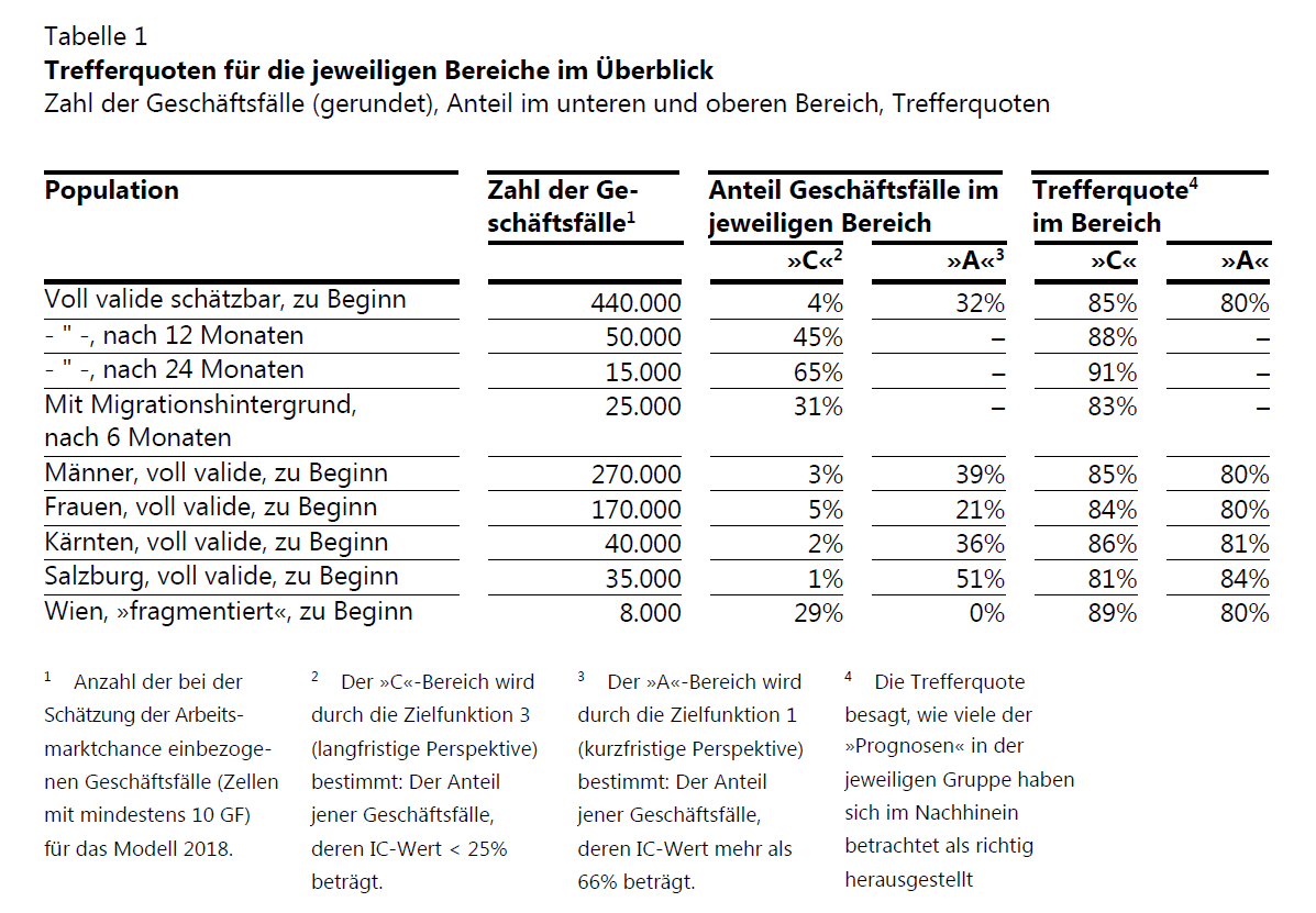
- What is shown here (and what isn’t)?
The Infamous “AMS-Algorithmus” IV
- The cut-off points were set (manually) at 25% for group C and 66% for group A
- By setting the cut-off points low for group C and high for group A, they achieved high precision in those two classes
- The precision in group B is not shown here, as well as other measures that would help us judge the predictive performance
Cross Validation
The real magic behind supervised machine learning
The Problem of Overfitting
- Models achieve an extremely good fit through the usage of many variables and high depth
- Danger of underestimating the random error \(\sigma^2\) of the data-generating process
- Results in a model with low in-sample prediction error but high out-of-sample error
The Solution to Overfitting
- Split your data into a training data set and a test data set
- The model is estimated using the training data, and performance measures are calculated using only the test data
- Repeat the process for different parameter values (e.g., for the penalty term \(\lambda\)) and choose the value which optimizes some performance measure over the test data
- This serves two purposes
- As a performance measure independent of the sample where the model was fit
- To choose hyperparameters such as \(\lambda\) (regularization)
Out of Sample Error
complexities = Array.from({ length: 10 }, (_, i) => i + 1);
trainingErrors = complexities.map(c => 2.5 / c + 0.5);
validationErrors = complexities.map(c => 1 + 0.2 + 0.15 * Math.pow(c - 5, 2));

error = ({
  style: { fontSize: "15px", backgroundColor: "transparent", padding: "20px" },
  height: 400,
  width: 500,
  x: {
    label: "Model complexity",
    ticks: [],
    axis: true
  },
  y: {
    label: "Error",
    ticks: [],
    axis: true
  },
  marks: [
    Plot.line(
      complexities.map((c, i) => ({ complexity: c, error: trainingErrors[i] })),
      { x: "complexity", y: "error", stroke: "#9C6B91", curve: "natural" }
    ),
    Plot.line(
      complexities.map((c, i) => ({ complexity: c, error: validationErrors[i] })),
      { x: "complexity", y: "error", stroke: "#336699", curve: "natural" }
    ),
    Plot.text(
      [{ complexity: 8.5, error: 1, text: "Training error" }],
      { x: "complexity", y: "error", text: "text", fill: "#9C6B91", dx: 10, dy: -10 }
    ),
    Plot.text(
      [{ complexity: 8.5, error: 2, text: "Validation error" }],
      { x: "complexity", y: "error", text: "text", fill: "#336699", dx: 10, dy: 10 }
    ),
    Plot.text(
      [{ text: "Underfitting\nHigh bias", complexity: 2.5, error: 4.5 }],
      { x: "complexity", y: "error", text: "text", fill: "black", dx: 5, dy: -10 }
    ),
    Plot.text(
      [{ text: "Overfitting\nHigh variance", complexity: 8.25, error: 4.5 }],
      { x: "complexity", y: "error", text: "text", fill: "black", dx: -5, dy: -10 }
    ),
    Plot.ruleX([1], { stroke: "black" }),
    Plot.ruleY([0])
  ]
});- Prediction will always be better in the training data
- Bias-Variance Trade-Off exists over model complexity
- Complexity means more parameters or a more flexible functional form
- number of predictors \(k\), leaves of a tree, weights of a network
- inverse of the shrinkage penalty \(\lambda\)
Types of Cross Validation
- Simple hold-out
- k-fold cross-validation
- LOOCV (leave-one-out cross-validation)
- LGOCV (leave-group-out cross-validation)
- OOB (out-of-bag samples)
- Time series-specific cross-validation (e.g., day-forward chaining)
k-Fold Cross Validation
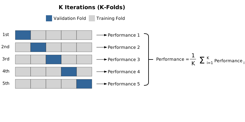
Properties of Cross Validation
- Training and testing environment should closely reflect the prediction problem to get an accurate expectation of prediction error
- Simple hold-out sample less suitable for optimization
- k-fold cross-validation gives downward-biased estimate of performance because it only utilizes the fraction \(\frac{k-1}{k}\) for training
- LOOCV gives approximately unbiased estimate of performance but has a higher variance
- LGOCV can be meaningful if the prediction problem tries to infer information from one group to another (e.g., countries, groups of people, etc.)
- Time-specific methods exclude future information in training
Benign Overfitting
- The classical picture says a model that overfits on training data generalizes badly
- However heavily overparameterized models with \(k \gg n\) routinely interpolate and predict well out of sample
- Test error follows a double descent curve: it peaks at the interpolation threshold \(k = n\) and falls again as \(k\) grows further
- Neural networks often are trained to near-zero training error yet still generalize well
A Perfect Summary II

Trees and CV in R
Putting it all together
Confusion Matrix in R
Confusion Matrix and Statistics

              Reference
Prediction     successful unsuccessful
  successful          468          298
  unsuccessful        260          544

               Accuracy : 0.6446
                 95% CI : (0.6203, 0.6683)
    No Information Rate : 0.5363
    P-Value [Acc > NIR] : <2e-16

                  Kappa : 0.2879

 Mcnemar's Test P-Value : 0.1173

            Sensitivity : 0.6429
            Specificity : 0.6461
         Pos Pred Value : 0.6110
         Neg Pred Value : 0.6766
             Prevalence : 0.4637
         Detection Rate : 0.2981
   Detection Prevalence : 0.4879
      Balanced Accuracy : 0.6445

       'Positive' Class : successful
Cut-Off in R
test$score_tree <- predict(
  tree,
  newdata = test,
  type = c("prob")
  )[,1]

test <- test |>
  mutate(prediction_tree = as.factor(ifelse(
    score_tree > 0.3 ,
    "successful",
    "unsuccessful"
    )))

confusion <- confusionMatrix(
  data = test$prediction_tree,
  reference = test$target_low,
  positive = "successful",
  mode = "sens_spec"
  )
Confusion Matrix and Statistics
Reference
Prediction successful unsuccessful
successful 565 466
unsuccessful 163 376
Accuracy : 0.5994
95% CI : (0.5746, 0.6237)
No Information Rate : 0.5363
P-Value [Acc > NIR] : 2.776e-07
Kappa : 0.2166
Mcnemar's Test P-Value : < 2.2e-16
Sensitivity : 0.7761
Specificity : 0.4466
Pos Pred Value : 0.5480
Neg Pred Value : 0.6976
Prevalence : 0.4637
Detection Rate : 0.3599
Detection Prevalence : 0.6567
Balanced Accuracy : 0.6113
'Positive' Class : successful
ROC- and PR-Curve in R
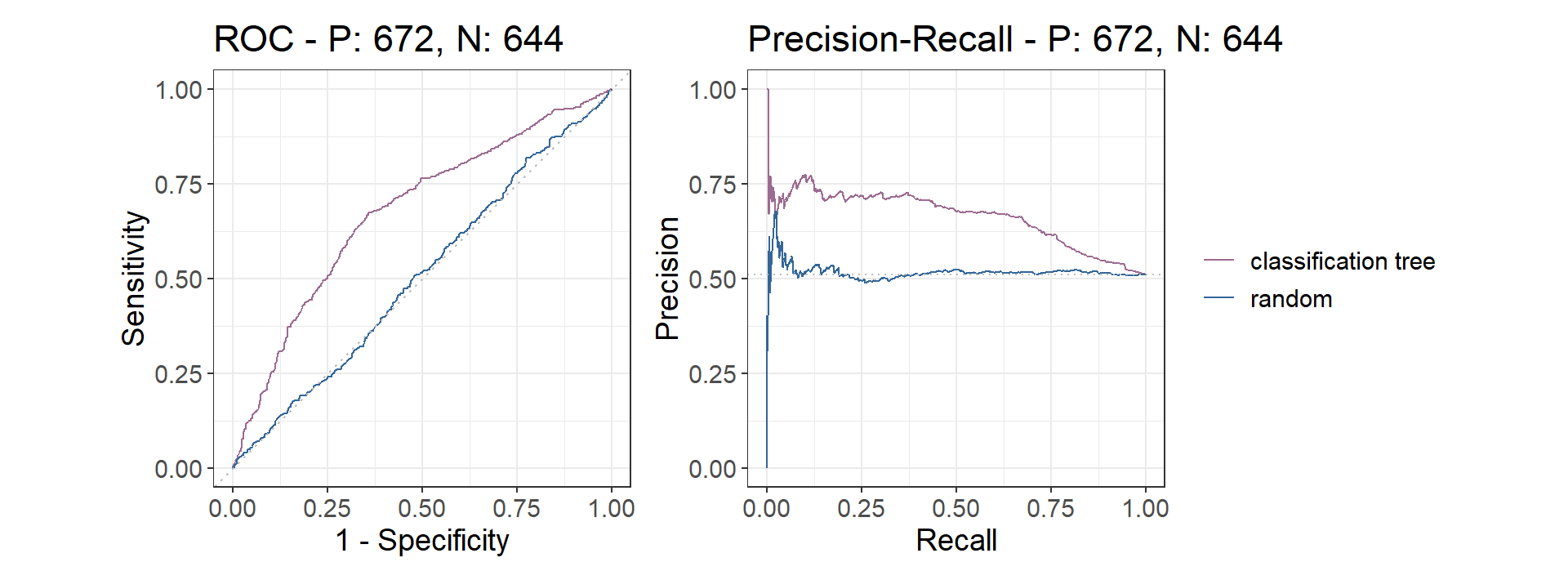
test$prediction_tree_scores <- predict(tree, test, type = c("prob"))[,2]
test$prediction_random <- runif(n = nrow(test))

precrec_obj <- evalmod(
  scores = cbind(test$prediction_tree_scores, test$prediction_random),
  labels = cbind(test$target_low, test$target_low),
  modnames = c("classification tree", "random"),
  ties_method = "first"
  )
CV in R - Caret
caret: classification and regression training
trControltakes care of the cross-validation processmethodhere specifies type of CVsummaryFunctionspecifies computation of performance measures
tuneGridchooses the parameters to try for the model
Training the Model
metricchooses what performance measure you want to optimizemethodspecifies the model, which can be implemented in some other package- Function will automatically choose the parameters which work best in the specified training and test process
CART

4830 samples
   3 predictor
   2 classes: 'successful', 'unsuccessful'

No pre-processing
Resampling: Cross-Validated (10 fold, repeated 10 times)
Summary of sample sizes: 4346, 4348, 4347, 4347, 4347, 4347, ...
Resampling results across tuning parameters:

  cp     ROC        Sens       Spec
  5e-04  0.7173981  0.6741891  0.6543656
  1e-03  0.7169620  0.7072193  0.6465661
  5e-03  0.6996839  0.6867633  0.6737720
  5e-02  0.6612506  0.7439858  0.5740977

ROC was used to select the optimal model using the largest value.
The final value used for the model was cp = 5e-04.
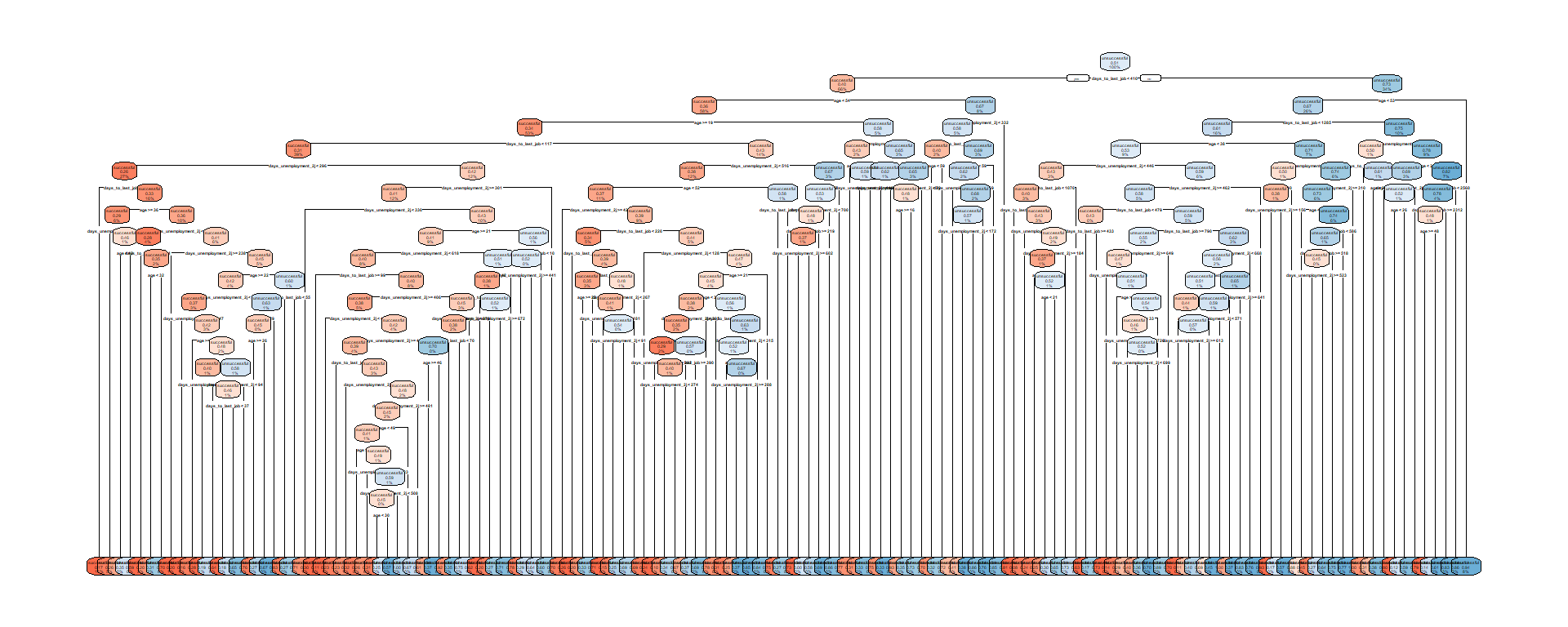
Extracting the Model
Predicting in Test Data
Confusion Matrix and Statistics

              Reference
Prediction     successful unsuccessful
  successful          409          235
  unsuccessful        234          438

               Accuracy : 0.6436
                 95% CI : (0.6171, 0.6695)
    No Information Rate : 0.5114
    P-Value [Acc > NIR] : <2e-16

                  Kappa : 0.2869

 Mcnemar's Test P-Value : 1

            Sensitivity : 0.6361
            Specificity : 0.6508
         Pos Pred Value : 0.6351
         Neg Pred Value : 0.6518
             Prevalence : 0.4886
         Detection Rate : 0.3108
   Detection Prevalence : 0.4894
      Balanced Accuracy : 0.6434

       'Positive' Class : successful
Model Comparison
test$prediction_caret_scores <- predict.train(
  tree_caret,
  test,
  type = c("prob"),
  na.action = na.pass
  )$unsuccessful

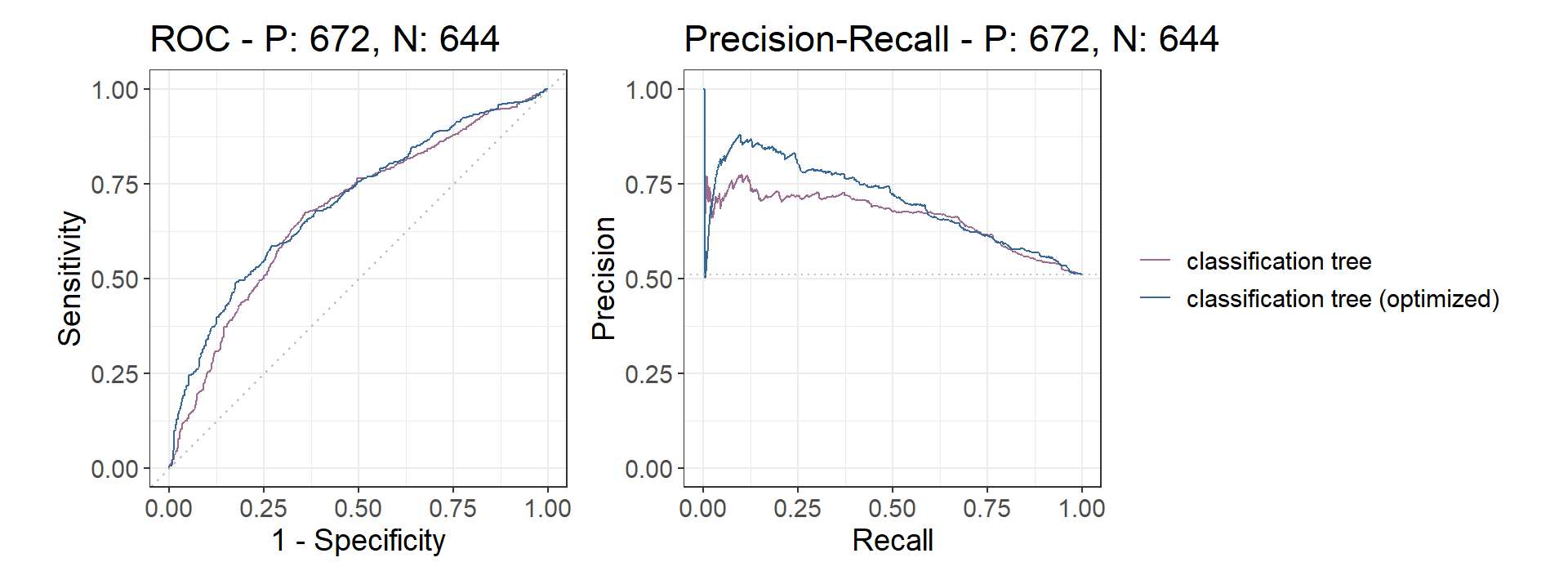
precrec_obj <- evalmod(
  scores = cbind(test$prediction_tree_scores, test$prediction_caret_scores),
  labels = cbind(test$target_low, test$target_low),
  modnames = c("classification tree", "classification tree (optimized)"),
  ties_method = "first"
  )